Adjoint Operators: The Grammar of Reality (Ep-2)

In Ivethium, our journey is never about memorizing definitions for their own sake, it is about uncovering the hidden machinery that nature seems to use to run itself. When we talk about operators and vectors, we are not just doing abstract math; we are building the grammar that describes reality. A particle’s wavefunction, a beam of light, the vibration of a bridge, even the state of an economy can be seen as vectors living in some space, acted upon by operators that evolve, measure, rotate, or filter them. To truly grasp how this works, we need to understand the adjoint: the operator’s mirror in the geometry of the space. Once we understand that relationship, a deeper symmetry emerges, one that splits spaces cleanly into orthogonal worlds and reveals the underlying order in systems that seem infinitely complex.

Note: If you are new to Ivethium, we recommend starting with these articles:
👉 Operators Basics
👉 The L2 Norm and Inner Products
👉 Cracking Hilbert Space

What Is an Adjoint Operator?

Before we dive into elegant theorems and applications, let's start with the most basic question: What exactly is an adjoint operator?

The Core Definition

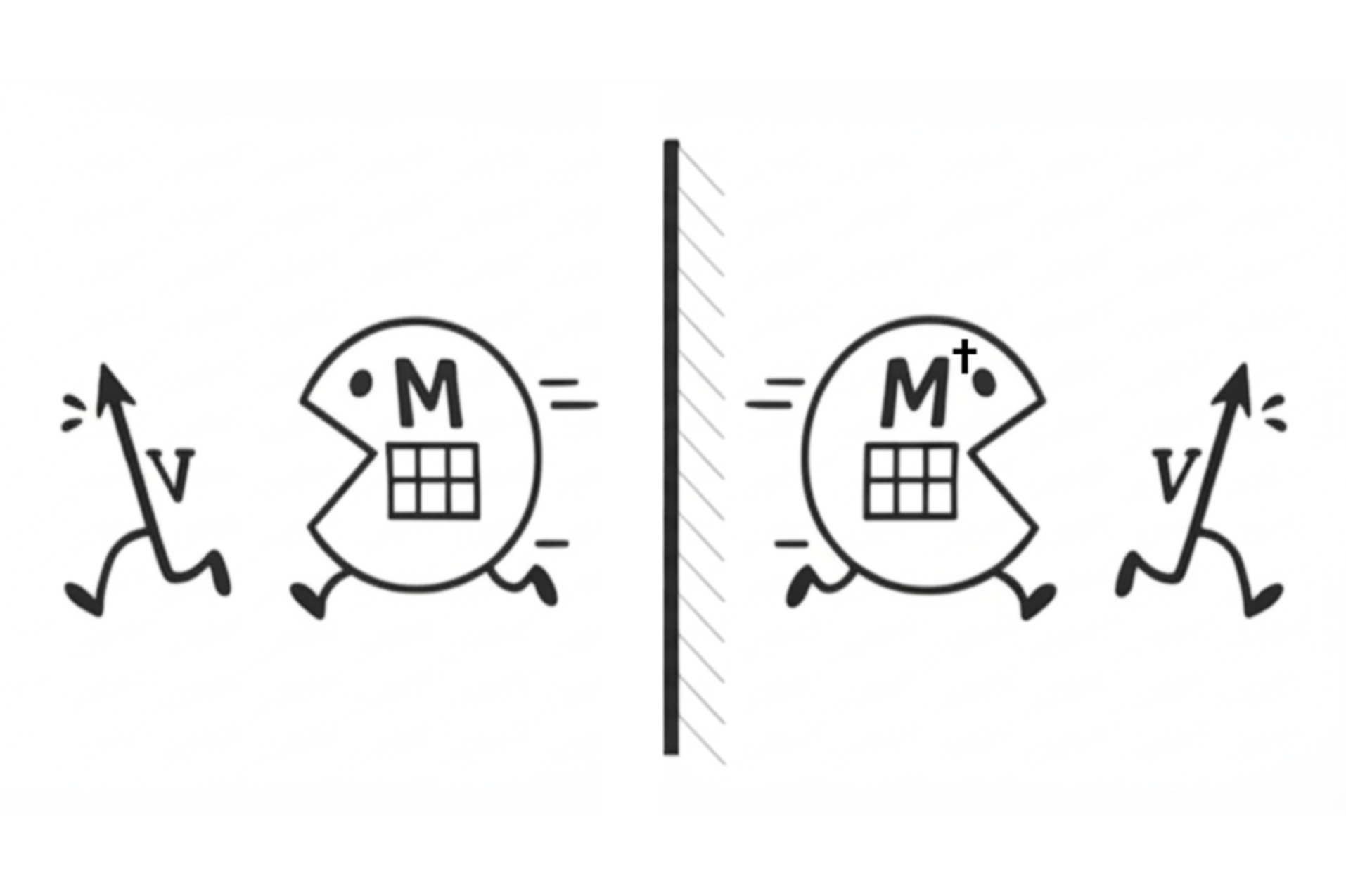
For any linear operator T on a Hilbert space (a vector space with an inner product), the adjoint operator T† is defined by this fundamental relationship:

$⟨Tx, y⟩ = ⟨x, T^{\dagger} y⟩$ for all vectors $x$, $y$

What This Actually Means

The adjoint T† is the unique operator that "moves" T from the left side of an inner product to the right side. Think of it as the operator that captures how T interacts with the geometry of the space.

In finite dimensions: The adjoint is simply the conjugate transpose of the matrix. For real matrices, this becomes just the transpose: $T{\dagger} = T^T$ .

A Simple Example

Let's see this with a concrete 2×2 matrix:

$$T = \begin{bmatrix} 2 & 1 \\ 0 & 3 \end{bmatrix}$$

The adjoint is:

$$T^{\dagger} = \begin{bmatrix} 2 & 0 \\ 1 & 3 \end{bmatrix}$$

Now let's verify the defining property with vectors $x = \begin{bmatrix} 1 \\ 0 \end{bmatrix}$ and $y = \begin{bmatrix} 1 \\ 1 \end{bmatrix}$:

• Left side: $\langle Tx, y \rangle = \left\langle \begin{bmatrix} 2 \\ 0 \end{bmatrix}, \begin{bmatrix} 1 \\ 1 \end{bmatrix} \right\rangle = 2$
• Right side: $\langle x, T^{\dagger}y \rangle = \left\langle \begin{bmatrix} 1 \\ 0 \end{bmatrix}, \begin{bmatrix} 2 \\ 1 \end{bmatrix} \right\rangle = 2$ ✓

Special Types of Operators

Now that we understand what an adjoint is, let's explore two crucial special cases that appear everywhere in mathematics and physics.

Self-Adjoint Operators (Hermitian)

An operator T is self-adjoint if it equals its own adjoint:

$$T = T^{\dagger}$$

What this means geometrically: The operator behaves symmetrically with respect to the inner product: $\langle Tx, y \rangle = \langle x, Ty \rangle$ for all vectors $x, y$.

Examples across different spaces:

1. Differential operator example: The second derivative operator on L²(ℝ):

$$T = -\frac{ d^2 }{ dx^2 }$$

This is self-adjoint on the space of square-integrable functions with appropriate boundary condition

2.Multiplication operator: On L²([0,1]), define (Mf)(x) = x·f(x):

$$\langle Mf, g \rangle = \int_0^1 x f(x) \overline{g(x)} dx = \int_0^1 f(x) x \overline{g(x)} dx = \langle f, Mg \rangle$$

So M is self-adjoint.

Key properties of self-adjoint operators (in any dimension):

• All eigenvalues are real numbers
• Eigenvectors/eigenfunctions for different eigenvalues are orthogonal.
  👉 We have not yet covered eigenvectors in Ivethium style discussions yet. This is going to appear in some of the most profound results that we will be discussing in the future posts.
• Admit spectral decomposition (generalization of diagonalization)
  👉 We'll discuss this under spectral theory in upcoming articles.
• They represent "measurements" or "observables" in quantum mechanics.
  👉 We're planning a dedicated series of articles on this topic.
• The spectral theorem applies: every self-adjoint operator can be "diagonalized" using a possibly continuous spectrum.
  👉 Diagonalization will be covered in detail in this episode. Don't worry about digging deeper right now. Just bookmark it for later.

Unitary Operators

An operator U is unitary if its adjoint equals its inverse:

$$U^{\dagger} = U^{-1} \text{ or equivalently } U^{\dagger}U = I$$

What this means geometrically: The operator preserves all distances and angles.

Examples across different spaces:

1. Finite-dimensional example:

$$R = \begin{bmatrix} 0 & -1 \\ 1 & 0 \end{bmatrix} \quad \Rightarrow \quad R^{\dagger}R = I \text{ (unitary)}$$

This rotates vectors by 90°:

• Acting on $\begin{bmatrix} 1 \\ 0 \end{bmatrix}$: $R\begin{bmatrix} 1 \\ 0 \end{bmatrix} = \begin{bmatrix} 0 \ 1 \end{bmatrix}$ (rotated, but same length)
• Acting on $\begin{bmatrix} 0 \\ 1 \end{bmatrix}$: $R\begin{bmatrix} 0 \\ 1 \end{bmatrix} = \begin{bmatrix} -1 \\ 0 \end{bmatrix}$ (rotated, but same length)

2. Fourier Transform on $L^2(\mathbb{R})$: The Fourier transform $F: L^2(\mathbb{R}) \to L^2(\mathbb{R})$ defined by:

$$(Ff)(\omega) = \int_{-\infty}^{\infty} f(t)e^{-2\pi i\omega t} dt$$

is unitary with $F^{\dagger} = F^{-1}$ (the inverse Fourier transform).

3. Translation operator: On $L^2(\mathbb{R})$, define $(T_a f)(x) = f(x - a)$:

$$\langle T_a f, T_a g \rangle = \int f(x-a)\overline{g(x-a)} dx = \int f(y)\overline{g(y)} dy = \langle f, g \rangle$$

Key properties of unitary operators (in any dimension):

• Preserve inner products: $⟨Ux, Uy⟩ = ⟨x, y⟩$ (General Parseval Identity)
• All eigenvalues lie on the unit circle in the complex plane
  👉 We will dig deeper into this, I promise!
• Preserve orthonormal bases (map them to orthonormal bases)
• They represent "rotations," "evolutions," or "isometries" that preserve structure
• Invertible with bounded inverse
• Form a group under composition

The Deep Connection to Orthogonality

Both self-adjoint and unitary operators have profound relationships with orthogonality (perpendicularity), but in different ways.

Self-Adjoint Operators and Orthogonality

The Guarantee: If T is self-adjoint, then eigenvectors corresponding to different eigenvalues are orthogonal. (As I mentioned before, we are going to dig deeper into eigenvectors. But till then, just consider the eigenvector's simple definition.)

Why this happens: Let's prove it!

Suppose:

• $Tv = λv$ (v is an eigenvector with eigenvalue λ)
• $Tw = μw$ (w is an eigenvector with eigenvalue μ)
• Say $λ ≠ μ$
• Then:
  $⟨Tv, w⟩ = λ⟨v, w⟩$ (since $Tv = λv$)
  $⟨Tv, w⟩ = ⟨v, Tw⟩$ (since $T = T†$)
  $⟨v, Tw⟩ = μ⟨v, w⟩$ (since $Tw = μw$)
• So: $λ⟨v, w⟩ = μ⟨v, w⟩$

👉 Since $λ ≠ μ$, we must have $⟨v, w⟩ = 0$, meaning $v ⊥ w$.

Unitary Operators and Orthogonality

The Guarantee: Unitary operators preserve all orthogonal relationships.

What this means: If $x ⊥ y$, then $Ux ⊥ Uy$.

Why this happens: Since $U^{\dagger} U = I$, we have:

$⟨Ux, Uy⟩ = ⟨x, U^{\dagger} Uy⟩ = ⟨x, y⟩$

So if $⟨x, y⟩ = 0$ (orthogonal), then $⟨Ux, Uy⟩ = 0$ (still orthogonal).

The Special Case: Both Self-Adjoint AND Unitary

Some operators are both self-adjoint and unitary. This creates something very special:

Example: Reflection matrix

$$A = \begin{bmatrix} 1 & 0 \\ 0 & -1 \end{bmatrix}$$

Check self-adjoint: $A = A^{\dagger}$ ✓
Check unitary: $A^{\dagger} A = A² = I$ ✓

What this means: $A² = I$, so applying the operator twice returns to the original vector. This is an involution (like flipping a coin).

Properties:

• Eigenvalues can only be $+1$ or $-1$
• Represents pure reflections without distortion

More Concrete Examples

Let's work through several examples across finite and infinite dimensions to see these concepts in action:

Self-Adjoint Examples

1. Projection onto x-axis (finite-dimensional):

$$P = \begin{bmatrix} 1 & 0 \\ 0 & 0 \end{bmatrix} \quad \Rightarrow \quad P = P^{\dagger} \text{ (self-adjoint)}$$

• Acting on $\begin{bmatrix} 3 \\ 4 \end{bmatrix}$: $P\begin{bmatrix} 3 \\ 4 \end{bmatrix} = \begin{bmatrix} 3 \\ 0 \end{bmatrix}$ (projects onto x-axis)
• Note: Not invertible (information is lost)

2. Stretching transformation (finite-dimensional):

$$S = \begin{bmatrix} 2 & 0 \\ 0 & 5 \end{bmatrix} \quad \Rightarrow \quad S = S^{\dagger} \text{ (self-adjoint)}$$

• Acting on $\begin{bmatrix} 1 \\ 1 \end{bmatrix}$: $S\begin{bmatrix} 1 \\ 1 \end{bmatrix} = \begin{bmatrix} 2 \\ 5 \end{bmatrix}$ (stretches along both axes)
• Eigenvalues: 2 and 5 (both real)

3. Laplacian operator (infinite-dimensional): On $L^2(\Omega)$ for a domain $\Omega$, the Laplacian $\Delta = \nabla^2$ is self-adjoint:

$$\langle \Delta f, g \rangle = \langle f, \Delta g \rangle \text{ (with appropriate boundary conditions)}$$

• Eigenvalues are negative real numbers
• Eigenfunctions form an orthogonal basis (like sines/cosines)

4. Multiplication by position (infinite-dimensional): On $L^2(\mathbb{R})$, the operator $(Xf)(x) = x \cdot f(x)$:

• Self-adjoint: $\langle Xf, g \rangle = \langle f, Xg \rangle$
• Continuous spectrum: all real numbers
• No normalizable eigenfunctions (only generalized ones)

Unitary Examples

1. 45° rotation (finite-dimensional):

$$R = \begin{bmatrix} \cos(\pi/4) & -\sin(\pi/4) \\ \sin(\pi/4) & \cos(\pi/4) \end{bmatrix} = \begin{bmatrix} \sqrt{2}/2 & -\sqrt{2}/2 \\ \sqrt{2}/2 & \sqrt{2}/2 \end{bmatrix}$$

• Preserves lengths and angles
• Eigenvalues: $e^{i\pi/4}$ and $e^{-i\pi/4}$ (on unit circle)

2. Complex phase shift (finite-dimensional):

$$U = \begin{bmatrix} i & 0 \\ 0 & i \end{bmatrix} \quad \Rightarrow \quad U^{\dagger}U = I \text{ (unitary)}$$

• Rotates all vectors by 90° in complex plane
• Eigenvalues: both equal to $i$

3. Fourier Transform (infinite-dimensional): $F: L^2(\mathbb{R}) \to L^2(\mathbb{R})$ is unitary with spectacular properties:

• Maps time domain to frequency domain
• $F^4 = I$ (applying it 4 times returns the original)
• Transforms convolution to multiplication

The Crown Jewel: The Fundamental Theorem

Now that we understand adjoints, self-adjoint operators, unitary operators, and their connections to orthogonality, we can appreciate one of the most beautiful theorems in linear algebra. But first, we need to understand some key concepts.

What Are Kernels and Ranges?

For any linear operator $T$, there are two fundamental subspaces that capture its essential behavior:

The Kernel (Null Space):

$ker(T) = {x : Tx = 0}$

The kernel is the set of all vectors that T "kills" (sends to zero).

The Range (Image):

$range(T) = {Tx : x in the domain}$

The range is the set of all vectors that T can "produce" (all possible outputs).

Some Examples:

1. Projection matrix:

$$P = \begin{bmatrix} 1 & 0 \\ 0 & 0 \end{bmatrix}$$

To find $\ker(P)$: We need $Px = 0$

$$\begin{bmatrix} 1 & 0 \\ 0 & 0 \end{bmatrix}\begin{bmatrix} x \ y \end{bmatrix} = \begin{bmatrix} 0 \\ 0 \end{bmatrix} \quad \Rightarrow \quad \begin{bmatrix} x \\ 0 \end{bmatrix} = \begin{bmatrix} 0 \\ 0 \end{bmatrix} \quad \Rightarrow \quad x = 0, \text{ } y \text{ can be anything}$$

So $\ker(P) = {(0, y) : y \in \mathbb{R}}$ (the y-axis)

To find $\text{range}(P)$: We see what $P$ can produce

$$P\begin{bmatrix} x \\ y \end{bmatrix} = \begin{bmatrix} 1 & 0 \\ 0 & 0 \end{bmatrix}\begin{bmatrix} x \\ y \end{bmatrix} = \begin{bmatrix} x \\ 0 \end{bmatrix} \quad \Rightarrow \quad P \text{ produces vectors of form } \begin{bmatrix} x \\ 0 \end{bmatrix}$$

So $\text{range}(P) = {(x, 0) : x \in \mathbb{R}}$ (the x-axis)

2. Rotation matrix:

$$R = \begin{bmatrix} 0 & -1 \\ 1 & 0 \end{bmatrix}$$

To find $\ker(R)$: We need $Rx = 0$

$$\begin{bmatrix} 0 & -1 \\ 1 & 0 \end{bmatrix}\begin{bmatrix} x \\ y \end{bmatrix} = \begin{bmatrix} 0 \\ 0 \end{bmatrix} \quad \Rightarrow \quad \begin{bmatrix} -y \\ x \end{bmatrix} = \begin{bmatrix} 0 \\ 0 \end{bmatrix} \quad \Rightarrow \quad y = 0 \text{ and } x = 0$$

So $\ker(R) = {0}$ (only kills the zero vector)

To find $\text{ range }(R)$: Since $R$ is invertible ($\det(R) = 1 \neq 0$), it can produce any vector

So $\text{ range }(R) = \mathbb{R}^2$ (can produce any vector)

3. Differential operator example: For $T = \frac{d}{dx}$ on smooth functions:

• $\ker(T) = {\text{constant functions}}$ (derivatives of constants are zero)
• $\text{range}(T) = {\text{all smooth functions}}$ (any smooth function is the derivative of something)

What is a Orthogonal Complement?

The orthogonal complement of a subspace S is:

$$S⊥ = {x : ⟨x, s⟩ = 0 for all s ∈ S}$$

Example: In ℝ³, if S is the xy-plane, then S⊥ is the z-axis.

The Fundamental Theorem

Theorem (Adjoint and Kernels): For any linear operator T:

$$ker(T{\dagger}) = (range(T))⊥$$
$$range(T{\dagger}) = (ker(T))⊥$$

What this means in plain English:

• The vectors that $T{\dagger}$ kills are exactly perpendicular to all vectors that $T$ can produce
• The vectors that $T{\dagger}$ produces are exactly perpendicular to all vectors that $T$ kills

Why This Is Beautiful

This theorem reveals that every linear operator creates a perfect orthogonal duality between what it does and what its adjoint does:

1. Every operator naturally splits space into orthogonal pieces
2. The adjoint provides the complementary perspective on this split
3. Orthogonality is the organizing principle that makes it all work

Example: The Derivative’s Two Perpendicular Worlds

We’re about to see something surprisingly elegant: the derivative operator doesn’t just measure rates of change, in the space of smooth periodic functions it actually splits the Hilbert space cleanly into two perpendicular worlds:

• Constant functions: perfectly flat, untouched by differentiation.
• Periodic functions with zero mean: pure oscillations, orthogonal to all constants.

This division is exact and orthogonal in the $L^2$ sense, and it falls right out of the Fundamental Theorem (Adjoint–Orthogonality Duality).

The space we are working in
A periodic function with period $L = b-a$ satisfies:
$$f(x+L) = f(x) \quad \forall x.$$
Constant functions are perfectly periodic, they trivially satisfy this for any $L$. In Fourier language, they are the zero-frequency mode. Our Hilbert space is:
$$\mathcal{H} = { f \in C^\infty([a,b]) \ :\ f(a) = f(b),\ f'(a) = f'(b), \dots }$$
smooth periodic functions on $[a,b]$.

The inner product
We measure angles and lengths in $\mathcal{H}$ using the $L^2$ inner product:
$$\langle f, g \rangle = \int_a^b f(x) , \overline{g(x)} , dx.$$

• The derivative operator
  Define:
  $$T = \frac{d}{dx}, \quad T : \mathcal{H} \to \mathcal{H}.$$

Kernel of $T$
If $f'(x) = 0$, $f$ is constant:
$$\ker(T) = {\text{constant functions}}.$$
These are the “flat” directions in $\mathcal{H}$.

The adjoint of $T$
Integration by parts:
$$\langle Tf, g \rangle = \left[ f(x)\overline{g(x)} \right]_a^b - \int_a^b f(x)\overline{g'(x)} , dx.$$
Periodic boundaries make the first term vanish, giving:
$$T^\dagger = -\frac{d}{dx}.$$

Range of $T^\dagger$
If $h = -g'(x)$ for some periodic $g$:
$$\int_a^b h(x) , dx = -\int_a^b g'(x) , dx = -(g(b)-g(a)) = 0.$$
So:
$$\operatorname{range}(T^\dagger) = {\text{smooth periodic functions with mean zero}}.$$

Orthogonal split
Take $c \in \ker(T)$ (a constant) and $h \in \operatorname{range}(T^\dagger)$ (mean-zero):
$$\langle c, h \rangle = c \int_a^b h(x) , dx = 0.$$
Thus:
$$\operatorname{range}(T^\dagger) = (\ker T)^\perp.$$
By the Fundamental Theorem:
$$\mathcal{H} = {\text{constants}} \ \oplus \ {\text{mean-zero periodic functions}}.$$

The picture
Every $f \in \mathcal{H}$ splits uniquely into:
$$f(x) = \bar{f} + \left(f(x) - \bar{f}\right)$$
where $\bar{f}$ is the constant part and $f(x) - \bar{f}$ is the mean-zero part.
Here
$$\bar{f} = \frac{1}{b-a} \int_a^b f(x) , dx.$$
The constant part is completely invisible to $T$; the mean-zero part is everything $T$ acts on. Differentiation is the knife that divides the space into these two perpendicular worlds.

where:
$$\bar{f} = \frac{1}{b-a} \int_a^b f(x) , dx.$$
The constant part is completely invisible to $T$; the mean-zero part is everything $T$ acts on. Differentiation is the knife that divides the space into these two perpendicular worlds.

Final Remark

The journey from "what is an adjoint?" to the beautiful theorem about kernels and ranges reveals the deep structure underlying linear algebra:

1. Adjoints capture how operators interact with inner product geometry
2. Self-adjoint operators create orthogonal eigenspaces with real eigenvalues
3. Unitary operators preserve all orthogonal relationships
4. The fundamental theorem shows how every operator and its adjoint create perfect orthogonal complements

This isn't just abstract mathematics. It's the foundation for understanding quantum mechanics, signal processing, optimization, and countless other areas where linear transformations meet geometry.

This mathematical framework points toward something even more profound. In our next posts, we'll explore how reality itself, from quantum particles to electromagnetic fields, from economic systems to neural networks, can be understood as nothing but operators acting on vectors. The adjoint relationships we've discovered here aren't just mathematical abstractions; they're the fundamental grammar of how the universe computes itself.