AM Radio as a Dot Product

In our previous posts, we established that signals are vectors living in an inner product space and explored how signal analysis is fundamentally about orthogonal decomposition of signals. In this article, we'll see how these abstract mathematical concepts come alive in one of the most ubiquitous technologies around us: AM radio.

The Mathematical Foundation We've Built

To recap our journey so far:

• We learned that signals can be treated as vectors in an infinite-dimensional space
• We discovered that inner product spaces give us the tools to measure "similarity" between signals
• We explored how orthogonal decomposition allows us to break down complex signals into simpler components

Now, let's see how AM radio is essentially a real-world implementation of these vector operations.

How AM Radio Waves Are Born: The Modulation Process

AM Radio Wave Creation

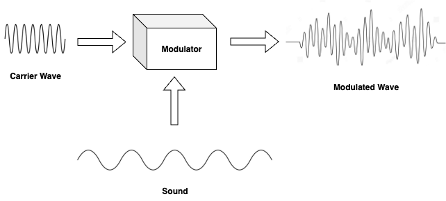
Before we dive into demodulation, let's understand how AM radio waves are created in the first place. At the radio station, the process begins with:

The Three Key Components

1. Audio Signal: The original audio $m(t)$ - music, voice, etc.
2. Carrier Wave: A high-frequency sinusoid $\cos(2\pi f_c t)$
3. Modulation: The audio modulates the amplitude of the carrier

The Transmitted Signal

The transmitted signal becomes:

$$s_{\text{transmitted}}(t) = [1 + m(t)] \cos(2\pi f_c t)$$

This equation shows how the audio signal $m(t)$ modulates the amplitude of the carrier wave, creating the AM (Amplitude Modulated) signal that gets transmitted through the air.

Notice how the audio signal $m(t)$ rides on top of the carrier frequency. The carrier provides the "vehicle" that can travel through space, while the audio information is encoded in the amplitude variations.

This modulation is the key to extraction - by encoding the audio as amplitude variations, we create a mathematical structure that can be reversed through dot product operations.

The Antenna Receives Everything: A Mixture of Signals

Radio Reception: Multiple Stations

When your radio antenna receives signals, it doesn't just pick up your desired station. The received signal $r(t)$ is actually a superposition of ALL radio stations broadcasting simultaneously:

$$r(t) = \sum_{i} A_i [1 + m_i(t)] \cos(2\pi f_i t + \phi_i)$$

Where:

• $A_i$ is the amplitude of station
• $m_i(t)$ is the audio from station
• $f_i$ is the carrier frequency of station
• $\phi_i$ is the phase offset

Your antenna is literally receiving a complex mixture containing jazz from 101.1 FM, talk radio from 880 AM, music from 1010 AM, and dozens of other stations all at once!

The Extraction Process: Mixing and Filtering

So how does your radio extract just one station from this chaotic mixture? The process involves two key steps:

Step 1: Mixing (Frequency Translation)

The received signal $r(t)$ is mixed (multiplied) with a locally generated carrier at the tune-in frequency $f_{\text{tune}}$:

$$mixed(t) = r(t) \cos(2\pi f_{\text{tune}} t)$$

This multiplication creates sum and difference frequencies for each station in the mixture.

Step 2: Low-Pass Filtering

The mixed signal is then passed through a low-pass filter that removes high-frequency components and keeps only the low-frequency (audio) information.

$$output(t) = LowPassFilter[mixed(t)]$$

How Traditional Engineering Explains This

In engineering schools, this process is typically explained using trigonometric identities, but let's be complete about it.

When we mix the received signal containing station $i$:

$$A_i [1 + m_i(t)] \cos(2\pi f_i t)$$

with our local oscillator $\cos(2\pi f_{\text{tune}} t)$, we get:

$$A_i [1 + m_i(t)] \cos(2\pi f_i t) \cos(2\pi f_{\text{tune}} t)$$

Using the trigonometric identity:

$$\cos(2\pi f_i t) \cos(2\pi f_{\text{tune}} t) = \frac{1}{2}[\cos(2\pi(f_i + f_{\text{tune}})t) + \cos(2\pi(f_i - f_{\text{tune}})t)]$$

This becomes:

$$A_i [1 + m_i(t)] \frac{1}{2}[\cos(2\pi(f_i + f_{\text{tune}})t) + \cos(2\pi(f_i - f_{\text{tune}})t)]$$

Now here's the key:

• If $f_i = f_{\text{tune}}$ (our desired station): The difference term becomes $\cos(2\pi(f_i - f_{\text{tune}})t) = \cos(0) = 1$, so after low-pass filtering we get $A_i [1 + m_i(t)] \frac{1}{2}$ - we recover the audio $m_i(t)$!

• If $f_i \neq f_{\text{tune}}$ (other stations): The difference term $\cos(2\pi(f_i - f_{\text{tune}})t)$ oscillates at frequency $|f_i - f_{\text{tune}}|$ and gets filtered out by the low-pass filter

Notice how the $[1 + m(t)]$ term is crucial - it's what carries the audio information through the entire process! The traditional trigonometric explanation often focuses on the carrier interaction but the modulation term is what makes the whole system work.

AM Radio: Dot Product at Work

But there's another way to think about this - one that connects directly to our vector space framework. The mixing and filtering process is actually computing the inner product between the received signal and a locally generated reference!

When you tune into your favorite AM radio station, what's happening under the hood is a beautiful demonstration of dot product computation. The AM demodulation process is literally computing the inner product between the received signal and a locally generated carrier wave.

The Demodulation Process: Inner Product in Action

The received AM signal can be written as:

$$s(t) = [1 + m(t)] \cos(2\pi f_ct)$$

Where:

• $m(t)$ is the modulating signal (audio)
• $f_c$ is the carrier frequency
• $\cos(2\pi f_ct)$ is the carrier wave

To extract the audio signal $m(t)$, the radio performs what's called synchronous detection or coherent demodulation. This involves:

1. Multiplying the received signal by a locally generated carrier: $\cos(2\pi f_ct)$
2. Integrating (or low-pass filtering) the result over a time window $T$

Mathematically, this is:

$$\text{output} = \frac{1}{T} \int_0^T s(t) \cos(2\pi f_ct) dt$$

This is exactly the definition of an inner product! We're computing the dot product between the received signal and the local carrier reference.

The mixing step is the multiplication, and the low-pass filtering is the integration (averaging) that computes the inner product. While engineering courses explain this through trigonometric identities, we can see it as an inner product operation in signal space - projecting the received signal onto the carrier direction.

The Critical Timing Relationships

Here's where the frequency domain intuition becomes crucial, and it directly relates to our previous discussion about orthogonal decomposition.

⚠️ Important Note for Advanced Readers: You might notice something important here. We're describing the demodulation as a simple dot product, but in reality, with a proper low-pass filter, what we're actually computing is a dot product with a weighted cosine function, where the weight function is time-shifting with t.

The actual operation is:

$$\text{output}(t) = \int_{-\infty}^{\infty} s(\tau) \cos(2\pi f_c \tau) h(t - \tau) , d\tau$$

Where $h(t)$ is the impulse response of the low-pass filter. Without this weight function, the correlation would be incomplete. The weighted cosine reference $\cos(2\pi f_c \tau) \cdot h(t - \tau)$ ensures proper correlation with the low-pass filtering characteristics.

This weighted, time-shifting approach is what allows us to continuously track the modulation $m(t)$ as it changes over time. We'll explore the deeper connections between convolution and dot products in a future article.

Carrier Frequency >> Modulation Spectrum

The carrier frequency $f_c$ is much higher than the highest frequency component in the modulating signal $m(t)$. For AM radio:

• Carrier frequencies: 540 kHz to 1700 kHz
• Audio bandwidth: typically 5 kHz maximum
• Ratio: $f_c/f_{\text{audio}} > 100:1$

This frequency separation is not accidental—it's what makes orthogonal decomposition possible.

Integration Window: The Key Parameter

The integration time window $T$ in our dot product computation must satisfy:

$$T \gg \frac{1}{f_c} \text{ (much longer than carrier period)}$$

$$T \ll \frac{1}{f_{\text{audio}}} \text{ (much shorter than audio variations)}$$

This choice of $T$ is what allows us to:

• Average out the high-frequency carrier oscillations
• Preserve the low-frequency modulation information

Why This Works: Orthogonality in Action

The magic happens because of orthogonality, and here's the key insight: since our integration window $T$ is much longer than the carrier period but much shorter than the modulation period, $[1 + m(t)]$ appears essentially constant during the integration time $T$.

This means our dot product becomes:

$$\int_0^T [1 + m(t)] \cdot \cos(2\pi f_c \cdot t) \cdot \cos(2\pi f_c \cdot t) , dt \approx [1 + m(t)] \cdot \int_0^T \cos^2(2\pi f_c \cdot t) , dt$$

Since $[1 + m(t)]$ is approximately constant over duration $T$, we can factor it out!

Now we're left with computing the dot product between two identical cosines:

$$\int_0^T \cos^2(2\pi f_c \cdot t) , dt$$

Here's the beautiful realization: when you're listening to an AM radio, you are literally tracing a dot product along time. Every moment of audio you hear is the result of a continuous dot product computation happening in your radio's circuitry. The music, the voice, the static - all are manifestations of inner product operations between the received electromagnetic waves and your radio's local oscillator.

As we discussed in our previous post, cosines of different frequencies are orthogonal when integrated from 0 to nT (where n is any integer). This is the fundamental reason why AM radio works:

• The dot product $\int \cos(2\pi f_c t) \cos(2\pi f_c t) , dt$ gives us a strong response (proportional to $T/2$)
• The dot product $\int \cos(2\pi f_c t) \cos(2\pi f_{\text{other}} t) , dt$ gives us zero when $f_c \neq f_{\text{other}}$

This is why other radio channels cancel out and we only hear our desired station! Each radio station uses a different carrier frequency, and the orthogonality of cosines at different frequencies ensures that:

• Our local oscillator (tuned to $f_c$) only responds to signals at frequency $f_c$
• All other stations at frequencies $f_{\text{other}}$ are orthogonal to our reference and contribute zero to the dot product

The result is:

$$\text{output} \approx [1 + m(t)] \frac{T}{2}$$

We've successfully extracted the modulation! The orthogonal cosine family has allowed us to selectively pick out our desired channel while rejecting all others.

The Vector Space Perspective

From our vector space viewpoint:

• The AM signal is a vector in signal space
• The local carrier $\cos(2\pi f_c t)$ is our reference vector
• The dot product measures the "component" of the received signal along the carrier direction
• The integration window $T$ acts as the window for our inner product in which $\cos$ functions behave as orthorgonal vectors

Practical Implications

This mathematical insight has profound practical consequences:

1. Synchronization: The local carrier must be perfectly synchronized with the transmitted carrier for optimal demodulation
2. Frequency Accuracy: Small frequency errors in the local oscillator directly affect the dot product result
3. Integration Time: The choice of $T$ represents a trade-off between carrier suppression and modulation fidelity

Demo Using Python

The following code demonstrates three AM Radio stations with sample audio signals and the entire demodulation process using our dot product (formally "inner product") approach. See how beautifully the signal can be reconstructed by tuning to the right radio station.

Conclusion

AM radio demodulation is a perfect example of how abstract mathematical concepts—vectors, inner products, and orthogonal decomposition—manifest in everyday technology. Every time you tune into an AM station, you're witnessing millions of dot product calculations per second, each one extracting a tiny piece of audio information from the electromagnetic spectrum.

The key insights that make this possible are:

• Carrier frequency >> modulation bandwidth (enabling orthogonal separation)
• Integration window >> carrier period (enabling carrier suppression)
• Integration window << modulation period (preserving audio information)

This beautiful interplay between frequency domain separation and time domain integration is what transforms the abstract mathematics of inner product spaces into the tangible experience of hearing music and voices transmitted through the air.