
Functions of Generators: Grammar of Reality (Ep-8)
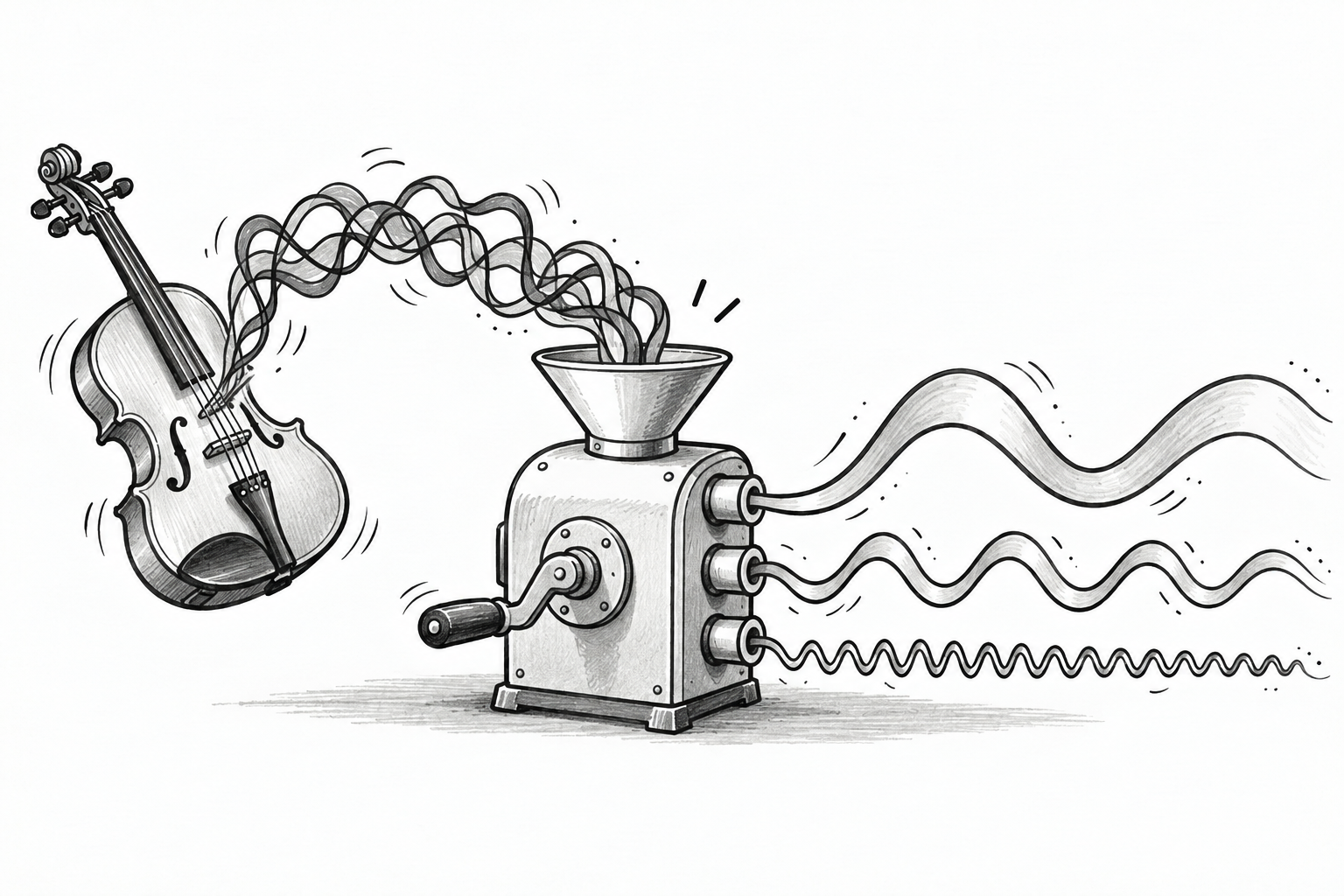
When a Rule Becomes the Input
In Episode 6, The Generators, we followed continuous change down to its instantaneous rule. After imposing linearity and working with a time-independent generator, we arrived at
$$\frac{dx}{dt}=Gx,\qquad x(t)=e^{tG}x(0).$$
In Episode 7, Projection Operators, we learned how to extract components belonging to eigenspaces.
Today, those two ideas meet.
Look again at the expression
$$e^{tG}.$$
We understand what $Gx$ means. A transformation acts on a state. But here the transformation itself appears to have become the input to another function.
We know how to calculate $e^3$. What could it mean to calculate an exponential of a rule?
Would $\sin(G)$ make sense too? Are we taking the sine of every matrix entry? Are we transforming the state? What kind of object comes out?
There is a precise answer. But writing down the answer too early hides the very thing we need to understand.
Let us build it.
A Function as a Recipe
Start with a deliberately simple function:
$$f(z)=2+3z+z^2.$$
Its instructions are visible. Square the input, add three times the input, then add two.
Operators already support addition, multiplication by scalars, and composition. We can therefore execute this recipe with an operator $G$:
$$f(G)=2I+3G+G^2.$$
Why $2I$ instead of $2$?
Because the result must act on states. The identity operator satisfies $Ix=x$, so $2I$ produces twice the original state.
Apply the whole expression to $x$:
$$f(G)x=2x+3Gx+G(Gx).$$
Now there is nothing mysterious to interpret. Keep twice the original state. Add three times a once-transformed copy. Add a twice-transformed copy.
Notice that $G^2$ means composition:
$$G^2x=G(Gx).$$
It does not mean squaring each matrix entry. The function's recipe is executed using operator multiplication.
For any polynomial,
$$p(z)=a_0+a_1z+\cdots+a_Nz^N,$$
we can construct
$$p(G)=a_0I+a_1G+\cdots+a_NG^N.$$
A rule has become the input to a larger recipe, and the result is another rule acting on the same state space.
But perhaps we have made the problem too easy.
What About Sine? What About Any Function?
A polynomial already consists of operations we know how to perform on operators.
What about
$$\sin(G)?$$
More generally, what could $f(G)$ mean when $f$ does not present itself as a finite list of additions and multiplications?
Some functions have a useful property: they can be represented by a power series.
For example,
$$\sin z=z-\frac{z^3 } {3!}+\frac{z^5} {5!}-\cdots,$$
and
$$e^z =1+z+\frac{z^2 } {2!}+\frac{z^3} {3!}+\cdots.$$
The factorial $n!$ means $1\cdot2\cdots n$. It supplies the weights in these particular recipes.
We now recognize the same operations as before. The recipe simply continues indefinitely.
To give that statement a precise meaning, first stop after finitely many terms:
$$S_1=G,$$
$$S_3=G-\frac{G^3} {3!},$$
$$S_5=G-\frac{G^3} {3!}+\frac{G^5} {5!}.$$
Each expression is an ordinary polynomial operator. For a finite-dimensional matrix $G$, this sequence converges as we include more terms. Its limit defines
$$\sin(G)=G-\frac{G^3} {3!}+\frac{G^5} {5!}-\cdots.$$
On a state,
$$\sin(G)x=Gx-\frac{G^3x} {3!}+\frac{G^5x} {5!}-\cdots.$$
We are combining repeated transformations with the coefficients belonging to sine.
Functions that equal a convergent power series around a point are called analytic there. Exponential, sine and cosine have series about zero that converge for every finite scalar input. Other functions have expansions that work only within a limited radius. Having derivatives of every order is not, by itself, enough to guarantee equality with a Taylor series.
So this construction comes with a condition. If
$$f(z)=\sum_{n=0}^{\infty} a_nz^n,$$
we define
$$f(G)=a_0I+\sum_{n=1}^{\infty} a_nG^n$$
when the operator series converges. For matrices, a sufficient condition is that an operator norm of $G$ lies within the scalar series' radius of convergence. Exponential, sine and cosine impose no such finite radius restriction.
We will develop the algebra first with finite-dimensional operators. Infinite-dimensional differential operators require additional care, which we will address when we return to the string.
There is also a small matter of units. A physical time generator carries units of inverse time. Its dimensionless combination is $tG$, as in $e^{tG}$ or $\sin(tG)$. We write $\sin(G)$ while discussing the algebra with units suppressed.
We have now made the notation meaningful.
But an infinite list of repeated transformations still leaves a question:
What does the resulting operator actually do?
Try One Extractor First
Episode 7 gave us an operator with an unusually simple property.
A projection $P$ extracts a component of a state. Extracting the same component twice changes nothing beyond the first extraction:
$$P^2=P.$$
Build an operator that extracts that component and scales it by a scalar $g$:
$$A=gP.$$
Its action is
$$Ax=gPx.$$
What happens when we apply it twice?
$$A^2x=gP(gPx).$$
Because $P$ is linear, the scalar can pass through:
$$A^2x =g2P2x=g^2Px.$$
Therefore,
$$A^2 =g^2P.$$
Once more:
$$A^3 =g^3 P^3 =g^3P.$$
The pattern is already visible.
The Projection Aha
From $P^2=P$, we obtain
$$P^3 =P^2P =PP=P,$$
and then
$$P^4 =P,\qquad P^5 =P,\qquad\ldots.$$
Thus
$$\boxed{P^n=P\quad\text{for every integer }n\geq1.}$$
Repeated scaling accumulates. Repeated extraction stops changing anything.
Consequently,
$$\boxed{(gP)n=gn P\quad(n\geq1).}$$
Both ingredients participated in the power. The number became $g^n$. The projector became $P^n$, which returned to $P$.
This is the mechanism we will need:
A projector can survive an entire series of repeated operations because every positive power returns the same extractor.
But keep the word positive. The zeroth power is the identity, and the identity preserves the entire state.
That small distinction has something to teach us.
Can We Pull the Projector Out of the Function?
Take our power-series recipe and apply it to the whole operator $gP$:
$$f(gP)=a_0I+a_1(gP)+a_2(gP)^2 +a_3(gP)^3 +\cdots.$$
Separate the scalar powers from the operator powers:
$$f(gP)=a_0I+a_1gP+a_2g^2 P^2 +a_3g^3 P^3 +\cdots.$$
Use the projection property:
$$f(gP)=a_0I+a_1gP+a_2g^2P +a_3g^3P +\cdots.$$
Now every term after the constant contains the same $P$. We can factor it out:
$$f(gP)=a_0I+\left(a_1g+a_2g^2 +a_3g^3 +\cdots\right)P.$$
The parentheses almost contain $f(g)$. They are missing $a_0$.
We cannot simply replace $a_0I$ with $a_0P$. One preserves the whole state; the other preserves only the selected component.
So where does the rest belong?
The Component We Have Been Leaving Behind
Every state can be written as
$$x=Px+(I-P)x.$$
The first term is what $P$ keeps. The second is what remains.
Indeed,
$$P(I-P)=P-P^2 =0.$$
So applying $P$ to that remainder gives zero.
The identity therefore splits as
$$I=P+(I-P),$$
and the constant term splits with it:
$$a_0I=a_0P+a_0(I-P).$$
Substitute this into our expression:
$$f(gP)=a_0P+a_0(I-P)+\left(a_1g+a_2g^2 +a_3g^3 +\cdots\right)P.$$
Group the terms multiplying $P$:
$$f(gP)=\left(a_0+a_1g+a_2g^2 +a_3g^3 +\cdots\right)P+a_0(I-P).$$
Now the first coefficient is exactly $f(g)$.
And what is $a_0$? Substitute zero into the original scalar series:
$$f(0)=a_0.$$
We have arrived at
$$\boxed{f(gP)=f(g)P+f(0)(I-P).}$$
The formula describes both parts of the space. On the selected component, $gP$ acts as multiplication by $g$. On the remaining component, it acts as zero. The function turns these values into $f(g)$ and $f(0)$.
For sine, $\sin(0)=0$, so
$$\sin(gP)=\sin(g)P.$$
For the exponential, $e^0 =1$, so
$$e^{gP} =e^g P+(I-P).$$
That extra identity action is real. The exponential preserves the component on which its generator is zero.
We can now answer the tempting question precisely: when $f(0)=0$,
$$f(gP)=f(g)P.$$
For a general function, we must also account for the complement.
Then What Is the Projector for Our Generator?
So far, we deliberately chose the simple operator $A=gP$.
A generator generally has more than one natural component. It can assign different values to different eigenspaces.
Recall the eigenspace decomposition from Episode 7. We now apply that construction to a generator that admits it:
$$G=\sum_{i=1}^{m}\left[g_iP_i\right].$$
For the next derivation, assume a finite-dimensional normal operator: one satisfying $GG\dagger=G\dagger G$. Such operators have a complete orthonormal eigenbasis. Hermitian and anti-Hermitian operators are included in this class.
This assumption lets us use exactly the mutually orthogonal eigenspace projectors already familiar from Episode 7:
$$P_i^2=P_i,\qquad P_iP_j=0\text{ for }i\neq j,\qquad \sum_{i=1}^{m}P_i=I.$$
We are not claiming that every generator has this structure.
What do the coefficients $g_i$ mean? Take a vector $v$ in the eigenspace selected by $P_i$. Then $P_iv=v$, and the other projectors give zero. Hence
$$Gv=g_iv.$$
The coefficient in front of each eigenspace projector is the corresponding eigenvalue.
The projector identifies the component. The eigenvalue specifies the action there.
Unlike the single-projector example, this collection covers the whole space. If the generator has a zero eigenspace, it is included in the collection too.
Do Not Distribute the Function by Guesswork
Looking at that sum, it is tempting to write
$$f\left(\sum_i g_iP_i\right)\stackrel{?}{=}\sum_i f(g_iP_i).$$
But functions do not generally distribute over addition.
Even squaring gives
$$(A+B)^2 =A^2 +AB+BA+B^2.$$
The middle terms do not disappear merely because we would like a simpler expression.
Nor is $f(gP)=f(g)f(P)$ a general rule.
We must execute the function's recipe on the complete operator, then allow the projection algebra to simplify the result.
Start with the square:
$$G^2 =\left(\sum_i g_iP_i\right)\left(\sum_j g_jP_j\right).$$
Expanding gives
$$G^2 =\sum_i\sum_j\left[g_ig_jP_iP_j\right].$$
When $i\neq j$, $P_iP_j=0$. When $i=j$, $P_i^2=P_i$. Therefore
$$G^2 =\sum_i\left[g_i^2P_i\right].$$
Repeating the argument gives
$$\boxed{G^n =\sum_i\left[g_i^n P_i\right]\quad(n\geq1).}$$
The same Aha now operates across the entire decomposition. Repeated extraction collapses within each component. Cross-products between different components vanish.
Two Sums, Two Different Jobs
Return to the function:
$$f(G)=a_0I+\sum_{n=1}^{\infty} a_nG^n.$$
There are now two indices to keep separate.
The index $n$ counts repeated applications: first power, second power, third power.
The index $i$ identifies eigenspaces.
Substitute the decomposition of each positive power, and use $I=\sum_iP_i$ for the constant:
$$f(G)=a_0\sum_iP_i+\sum_{n=1}^{\infty} a_n\sum_i\left[g_i^n P_i\right].$$
Since the eigenspace sum is finite and our power series converges, we may collect all contributions belonging to each fixed $i$:
$$f(G)=\sum_i\left[a_0P_i+\sum_{n=1}^{\infty} \left[a_ng_i^n P_i\right]\right].$$
For a fixed eigenspace, every power contains the same $P_i$. It can therefore come outside the sum over $n$:
$$f(G)=\sum_i\left[\left(a_0+\sum_{n=1}^{\infty} a_ng_i^n \right)P_i\right].$$
Notice the brackets.
The projector is outside the sum over powers, but remains inside the sum over eigenspaces.
It does not depend on $n$. It does depend on $i$.
The scalar expression in parentheses is the original function evaluated at $g_i$. Consequently,
$$\boxed{f(G)=\sum_i\left[f(g_i)P_i\right].}$$
Nothing in this calculation selectively protected the projectors. They participated in every power. Their algebra returned them in a form we could factor out.
And the constant term was never discarded. Completeness distributed it across the whole space.
This is why the full formula works even when $f(0)\neq0$.
An Infinite Operator Recipe Becomes Ordinary Scalar Mathematics
The result immediately gives
$$\sin(G)=\sum_i\left[\sin(g_i)P_i\right],$$
$$\cos(G)=\sum_i\left[\cos(g_i)P_i\right],$$
and
$$e^{tG} =\sum_i\left[e^{tg_i}P_i\right].$$
Instead of following an infinite series of operator powers, we evaluate familiar scalar functions and attach their results to the corresponding projectors.
The coefficients are also the eigenvalues of the new operator. For a vector $v$ in the $i$-th eigenspace,
$$f(G)v=f(g_i)v.$$
The original eigenspaces remain invariant. Different original eigenvalues may become the same number under $f$, in which case their subspaces belong to a larger shared eigenspace of $f(G)$.
This construction is called a functional calculus: a consistent way to build functions of operators.
Once a complete finite spectral decomposition is available, it also gives a way to define functions that have no useful Taylor series. We assign a well-defined scalar value $f(g_i)$ at every eigenvalue and assemble the operator from those values. Where the power-series construction applies, we have just proved that the two constructions agree.
For example, choosing the value $1$ on one selected eigenvalue and $0$ on the others recovers its eigenspace projector.
There are limits. The inverse requires nonzero eigenvalues. Logarithms and square roots may require specifying a branch. Non-diagonalizable operators contain information that eigenvalues alone do not capture. Continuous spectra require the spectral-measure machinery promised in Episode 7; that is a further extension, not a condition we need for this finite derivation.
Return to Episode 6: The Weights of Time
For a time-independent generator in our spectral setting,
$$U(t)=e^{tG} =\sum_i\left[e^{tg_i}P_i\right].$$
Apply it to the initial state:
$$\boxed{x(t)=\sum_i\left[e^{tg_i}P_ix(0)\right].}$$
Each initial component $P_ix(0)$ receives its own time-dependent multiplier.
If $g_i=a_i+ib_i$, then
$$e^{tg_i} =e^{a_it} e^{ib_it}.$$
The real part $a_i$ controls exponential growth or decay. The imaginary part $b_i$ controls phase rotation. A zero eigenvalue gives a stationary component.
This is a mathematical decomposition of the evolution. We need not imagine nature physically extracting components and then assembling them again.
At zero time, every exponential equals one:
$$U(0)=\sum_iP_i=I.$$
The resolution of identity from Episode 7 has become the zero-time case of evolution.
For example, with time measured in chosen units, suppose
$$G=-P_1+2P_2.$$
Then
$$U(t)=e^{-t} P_1+e^{2t} P_2.$$
The first component decays; the second grows. We can read that behaviour directly from two scalar exponentials.
But let us return to something we can hear.
The Violin Comes Back
In Episode 4's violin example, we used an ideal string with fixed ends and a wave speed $c$. Its transverse displacement $u(x,t)$ satisfies
$$u_{tt}=c^2 u_{xx},\qquad u(0,t)=u(L,t)=0.$$
This is the ideal undamped, unforced string model. It describes free vibration after release, rather than the full interaction of a continuously bowed violin with its body.
Let us call the spatial operator $\mathcal A$, keeping $L$ for the string length:
$$\mathcal A=-\frac{\partial^2}{\partial x^2}.$$
Its normalized fixed-end modes are
$$\phi_n(x)=\sqrt{\frac{2}{L}}\sin\left(\frac{n\pi x}{L}\right).$$
Differentiating twice shows
$$\mathcal A\phi_n=\lambda_n\phi_n,\qquad \lambda_n=\left(\frac{n\pi}{L}\right)^2.$$
Normalization makes the inner-product extraction simple. As in Episode 7, define
$$(P_nw)(x)=\phi_n(x)\int_0^L\phi_n(s)w(s),ds.$$
Here $w$ is a string profile and $s$ is the integration variable. The integral finds its $n$-th mode coefficient; multiplication by $\phi_n(x)$ restores that component as a full profile.
Thus $P_n$ is the harmonic extractor we already understand.
What does time do to the extracted component?
Derive the Time Weight of One Harmonic
Write one vibrating mode as
$$u_n(x,t)=q_n(t)\phi_n(x),$$
where $q_n(t)$ is its changing amplitude.
Substitute into the wave equation. The time derivatives act on $q_n$; the spatial derivatives act on $\phi_n$:
$$\ddot q_n(t)\phi_n(x)=-c^2\lambda_nq_n(t)\phi_n(x).$$
Equating the mode coefficients gives
$$\ddot q_n=-c^2\lambda_nq_n.$$
Define its angular frequency by
$$\omega_n=c\sqrt{\lambda_n}=\frac{n\pi c}{L}.$$
The equation is therefore
$$\ddot q_n=-\omega_n^2q_n.$$
Sine and cosine enter because their second derivatives return minus themselves multiplied by $\omega_n^2$. With initial amplitude $q_n(0)$ and initial rate $\dot q_n(0)$, the solution is
$$q_n(t)=q_n(0)\cos(\omega_nt)+\frac{\dot q_n(0)}{\omega_n}\sin(\omega_nt).$$
Check the factor $1/\omega_n$: differentiating the sine term produces $\dot q_n(0)\cos(\omega_nt)$, which has exactly the required initial rate.
Nothing about the time weights has been guessed. They solve the modal equation and match its two initial conditions.
A Vibrating Shape as a Sum of Weighted Projections
Let
$$u_0(x)=u(x,0),\qquad v_0(x)=u_t(x,0).$$
The projector extracts
$$P_nu_0=q_n(0)\phi_n,\qquad P_nv_0=\dot q_n(0)\phi_n.$$
Multiplying each modal solution by its shape and adding the modes gives
$$\boxed{u(t)=\sum_{n=1}^{\infty}\left[\cos(\omega_nt)P_nu_0+\frac{\sin(\omega_nt)}{\omega_n}P_nv_0\right].}$$
Here $u(t)$ denotes the entire spatial profile at time $t$.
If we release the displaced string from rest, then $v_0=0$:
$$\boxed{u(t)=\left(\sum_{n=1}^{\infty}\left[\cos(\omega_nt)P_n\right]\right)u_0.}$$
Each harmonic of the initial shape is multiplied by its own cosine. Their sum gives the changing string.
This is the utility of the representation made visible: the complicated motion of a whole shape becomes ordinary scalar oscillations attached to fixed component extractors.
At $t=0$,
$$\cos(\omega_n0)=1,$$
so completeness returns the initial shape:
$$u(0)=\sum_nP_nu_0=u_0.$$
The Operator Function Hidden in the Sound
We have the positive spatial eigenvalues $\lambda_n$ and frequencies $\omega_n=c\sqrt{\lambda_n}$.
Define an operator $\Omega$ that assigns each harmonic its frequency:
$$\Omega=\sum_n\left[\omega_nP_n\right].$$
This is the spectral meaning of writing
$$\Omega=c\sqrt{\mathcal A}.$$
The square root acts on each positive eigenvalue of $\mathcal A$. It assigns $\sqrt{\lambda_n}$ to the same harmonic.
Applying cosine to $\Omega$ then gives
$$\cos(t\Omega)=\sum_n\left[\cos(t\omega_n)P_n\right].$$
Similarly, because the fixed-end frequencies are nonzero,
$$\Omega^{-1}\sin(t\Omega)=\sum_n\left[\frac{\sin(t\omega_n)}{\omega_n}P_n\right].$$
Our string solution becomes
$$\boxed{u(t)=\cos(t\Omega)u_0+\Omega^{-1}\sin(t\Omega)v_0.}$$
We have now encountered square roots, sine and cosine of operators in a single physical calculation, with each expression built from its action on the modes.
For the infinite string-mode system, these functions are defined through their spectral action. We do not assume that a Taylor series of an unbounded differential operator can act term by term on every profile. One may first retain finitely many harmonics, where our matrix calculations apply directly, and then take the modal limit. For finite-energy initial data the evolution has the appropriate norm convergence; pointwise differentiations require additional regularity.
But Where Is the Exponential?
Episode 6 used $e^{tG}$. The string shape has given us sine and cosine.
The reason is already present in the initial conditions. The wave equation requires both $u_0$ and $v_0$. A shape alone does not tell us whether the string is moving upward or downward.
To write a first-order evolution, collect both quantities:
$$X(t)=\begin{pmatrix}u(t)\v(t)\end{pmatrix},\qquad v=u_t.$$
Their derivatives are
$$u_t=v,\qquad v_t=-\Omega^2u.$$
Therefore
$$\frac{dX}{dt}=GX,\qquad G=\begin{pmatrix}0&I; -\Omega^2&0\end{pmatrix}.$$
We have obtained this generator simply by rewriting the two evolution rules.
The spatial operator $\mathcal A$ and the time generator $G$ are different objects. The former acts on a shape; the latter acts on shape and velocity together.
Consider just one harmonic, whose state is
$$X_n=\begin{pmatrix}q_n\\dot q_n\end{pmatrix}.$$
Its generator is the ordinary matrix
$$G_n=\begin{pmatrix}0&1\ ;-\omega_n^2&0\end{pmatrix}.$$
Multiplying it by itself gives
$$G_n^2 =-\omega_n^2 I_2,$$
where $I_2$ is the two-dimensional identity. Hence its even and odd powers are
$$G_n^{2k} =(-1)^k \omega_n^{2k} I_2,\qquad G_n^{2k+1} =(-1)^k \omega_n^{2k} G_n.$$
Separate the exponential series into those two groups:
$$e^{tG_n} =\left(1-\frac{\omega_n^2 t^2} {2!}+\cdots\right)I_2+\left(t-\frac{\omega_n^2 t^3} {3!}+\cdots\right)G_n.$$
Recognizing the scalar series gives
$$e^{tG_n}=\cos(\omega_nt)I_2+\frac{\sin(\omega_nt)}{\omega_n}G_n.$$
Substitute the matrix:
$$\boxed{e^{tG_n} =\begin{pmatrix}\cos(\omega_nt)&\sin(\omega_nt)/\omega_n\ -\omega_n\sin(\omega_nt)&\cos(\omega_nt)\end{pmatrix}.}$$
The first row gives the displacement formula we already derived. The second gives its velocity.
The exponential and the trigonometric description are now visibly the same evolution.
Can We Also Recover Exponential-Weighted Projectors?
Yes. We can construct them rather than introduce new symbols without explanation.
The characteristic equation of $G_n$ is
$$\det(G_n-gI_2)=g^2 +\omega_n^2=0.$$
Its two complex eigenvalues are therefore
$$g_{n,+}=i\omega_n,\qquad g_{n,-}=-i\omega_n.$$
To find their projectors, scale $G_n$ to an operator whose square is the identity:
$$B_n=\frac{G_n}{i\omega_n},\qquad B_n^2=I_2.$$
Then define
$$R_{n,+}=\frac{I_2+B_n}{2},\qquad R_{n,-}=\frac{I_2-B_n}{2}.$$
Why these combinations? Squaring the first gives
$$R_{n,+}^2 =\frac{I_2+2B_n+B_n^2} {4}=\frac{I_2+B_n}{2}=R_{n,+}.$$
The same holds for $R_{n,-}$, while
$$R_{n,+}R_{n,-}=\frac{I_2-B_n^2} {4}=0,\qquad R_{n,+}+R_{n,-}=I_2.$$
Moreover, $G_n=i\omega_nB_n$, so
$$G_nR_{n,+}=i\omega_nR_{n,+},\qquad G_nR_{n,-}=-i\omega_nR_{n,-}.$$
They are precisely the two eigenspace projectors. Our projection algebra now gives
$$\boxed{e^{tG_n} =e^{i\omega_nt} R_{n,+}+e^{-i\omega_nt} R_{n,-}.}$$
These projectors act on a harmonic's displacement–velocity pair, not on its spatial shape alone. In the unscaled coordinates they need not be orthogonal in the ordinary Euclidean inner product; their idempotence, vanishing cross-products and completeness are what the calculation uses.
For the whole string, first use $P_n$ on both initial profiles to isolate harmonic $n$, then apply $R_{n,+}$ or $R_{n,-}$ to that harmonic's pair. Call these combined operations $\Pi_{n,+}$ and $\Pi_{n,-}$. Summing over all harmonics gives
$$\boxed{U(t)=\sum_{n=1}^{\infty} \left[e{i\omega_nt}\Pi_{n,+}+e{-i\omega_nt} \Pi_{n,-}\right].}$$
Real initial data produce conjugate pairs, whose sum is the real vibration. The complex exponentials are another representation of the sine and cosine motion.
We have reached the exact format we wanted: time evolution as a sum of projection operators weighted by exponentials of the generator's eigenvalues.
What Counts as a State?
The algebra has completed its journey.
We began with a polynomial recipe. Power series extended that recipe to functions such as sine and exponential. Projection algebra then revealed why repeated operator actions could be collected into scalar functions of eigenvalues.
The projectors did not escape the function. They survived its powers.
Then the violin exposed something deeper. Its shape was enough to ask which harmonics were present. Its shape was not enough to predict what happened next. We had to include its velocity.
That choice changed the operator we needed. The spatial harmonic extractor and the full evolution projector were related, but they acted on different descriptions.
So before we ask which generator a physical system obeys, another question deserves its own chapter.
What information must a state retain?
Why position and velocity in one description, position and momentum in another? When does time itself need to be included? When do two different lists of numbers describe the same physical situation?
Next: What Counts as a State? — Choosing State Spaces for Physical Systems.