Generalizing AI as a Compression Algorithm

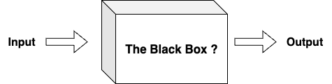
The Black Box Perspective

Imagine AI as a black box. You feed something in, and something comes out. It’s that simple on the surface — input goes in, output emerges. But what’s happening inside that box is far more fascinating than it first appears.

Think of this relationship as a massive map where each possible input connects to one or more outputs. Every question you could ask, every image you could show, every piece of text you could provide — all mapped to their corresponding responses, classifications, or transformations.

Here’s the crucial insight: since both inputs and outputs have maximum possible sizes in any practical system, the total number of possible input-output combinations is finite. Large, yes — astronomically large — but finite nonetheless. Every possible conversation, every possible image recognition task, every possible translation could theoretically be pre-computed and stored in one giant lookup table.

The Impossibly Large Table

Let’s say we wanted to build this complete input-output table. For a system that processes text, we’d need to account for every possible sequence of characters up to some maximum length. For images, every possible combination of pixel values. The memory requirements would be staggering — we’re talking about storage needs that would dwarf all the data centers on Earth combined.

This theoretical table would be the perfect AI: instant responses, no computation needed, just lookups. But here’s the fascinating part — from the outside, this lookup table would appear indistinguishable from the most sophisticated AI we could imagine. Ask it about quantum physics, show it an image, request a poem — it delivers perfect responses instantly.

This reveals something profound: intelligence, from a functional perspective, might just be about producing the right outputs for given inputs. The internal mechanism becomes irrelevant to the end user. But of course, this theoretical table is completely impractical. The storage requirements make it impossible to build or maintain.

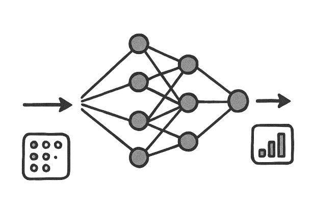
Enter Neural Networks: Compression in Action

Neural networks accomplish something remarkable: they perform essentially the same input-output mapping function, but using a drastically smaller number of parameters — what we call weights. Instead of storing every possible input-output pair, they learn to approximate this massive table using just millions or billions of weights rather than the quintillions of entries the full table would require.

By definition, neural networks exist in a compressed state compared to the uncompressed lookup table. Where the full table would require astronomical storage, neural networks achieve functionally equivalent behavior using orders of magnitude fewer parameters. The weights in a neural network are nothing more than a compact encoding of the same input-output relationships that would otherwise require that impossibly large table.

Noise as the True Driver of Lossy Compression?

Here’s where the story gets fascinating: neural network training is fundamentally driven by noise, and neural networks are essentially lossy compression systems. Could noise be the true engine that drives lossy compression?

The standard explanation for mini-batch gradient descent is computational efficiency and approximation:

w_new​ = w_old​ − α ∇ L_batch​(w)

where we approximate the full gradient with a smaller batch. This is typically framed as a necessary compromise — we accept some noise in our gradient estimates to make training computationally feasible.

But there may be a different way to look at this. What if the noise isn’t just an unfortunate side effect, but the actual mechanism driving compression? Consider the equation with explicit noise:

w_new​ = w_old​ − α (∇ L_batch​(w) + ϵ)

This noise ϵ comes from stochastic sampling, random initialization, and various training procedures. Instead of viewing this as approximation error, we could view it as the driver of the compression process itself.

When we think of neural networks as lossy compression systems — taking high-dimensional inputs and compressing them into compact representations that preserve only task-relevant information — many aspects of neural network optimization become strikingly similar to compression algorithms. The randomness forces the network to find representations robust to perturbations, naturally leading to more compressed, generalizable solutions that discard irrelevant details while preserving essential patterns.

This suggests a provocative hypothesis: noise might be the fundamental mechanism that enables lossy compression in neural networks. The randomness doesn’t just help with optimization — it actively drives the compression process by forcing the system to find representations that are robust to perturbations, which naturally leads to more compressed, generalizable solutions.

This is something worth considering deeply. If true, it would mean that the noise we often view as an unfortunate necessity of practical training is actually the core mechanism that makes neural network compression possible.

Random Walks as Drivers in Optimization

This perspective — that noise might be the fundamental mechanism rather than just a computational convenience — extends to many optimization problems where finding efficient solutions is the goal.

Consider Simulated Annealing, where the traditional explanation is that we’re mimicking physical cooling processes. But we could reframe this: the algorithm uses controlled random walks to explore solution spaces, and the “temperature” parameter controls how much noise to inject. Rather than just avoiding local optima, the noise might be actively driving the system toward more compressed, efficient solutions.

Monte Carlo methods are typically explained as ways to approximate intractable integrals through random sampling. But another view: the randomness enables these algorithms to discover compact representations of complex systems — essentially finding compressed solutions that capture essential behavior with far fewer parameters than exhaustive approaches.

Genetic Algorithms are usually framed as biological metaphors with random mutations and crossover. Alternatively: the noise from these random operations drives the evolution toward increasingly efficient solutions that compress the essence of successful strategies while discarding unnecessary complexity.

Even beyond neural networks, Stochastic Gradient Descent is commonly justified as a computational approximation. But perhaps the stochastic component isn’t just helping escape local minima — it might be the mechanism that enables algorithms to find compressed representations of the underlying optimization landscape.

In each case, we typically explain the random component as helpful for exploration or computational necessity. But what if we’re missing the deeper story? The noise might be the engine that drives these algorithms toward solutions that naturally compress complex problems into their essential components.

The Information Bottleneck Connection

This perspective finds compelling support in Naftali Tishby’s groundbreaking work on the Information Bottleneck principle. Tishby showed that optimal learning involves finding the best tradeoff between compression and prediction accuracy. Mathematically, this can be expressed as minimizing:

I(X; T) — β * I(T; Y)

where I(X; T) represents the mutual information between input X and compressed representation T, I(T; Y) represents the mutual information between the representation and output Y, and beta controls the compression-accuracy tradeoff.

Tishby discovered that deep learning proceeds in two distinct phases: a fitting phase where networks learn to predict labels, followed by a compression phase where they learn to “forget” irrelevant details. Crucially, he found that this compression phase — driven by the stochastic nature of gradient descent — is what enables generalization.

The stochastic gradient descent equation:

w_new = w_old — α ∇ L(w) + stochastic_noise

isn’t just an approximation of true gradient descent. According to Tishby’s framework, the stochastic noise is what drives the network toward the information bottleneck bound — the optimal compression that preserves only relevant information while discarding everything else.

This suggests that our reframing might be more than just a different perspective. If Tishby is correct, then noise isn’t incidental to compression in neural networks — it’s the fundamental mechanism that enables them to find optimal compressed representations. The randomness we introduce through stochastic training might be the key that unlocks the compression process itself.

Perhaps it’s time we stopped thinking of noise as something to tolerate in our algorithms, and started recognizing it as the engine of compression that makes learning possible.

References

1. Tishby, N., Pereira, F. C., & Bialek, W. (1999). The information bottleneck method. arXiv preprint physics/0004057.
2. Tishby, N., & Zaslavsky, N. (2015). Deep learning and the information bottleneck principle. arXiv preprint arXiv:1503.02406.
3. Shwartz-Ziv, R., & Tishby, N. (2017). Opening the black box of deep neural networks via information. arXiv preprint arXiv:1703.00810.
4. Schwartz-Ziv, R., & Tishby, N. (2017). “New Theory Cracks Open the Black Box of Deep Learning.” Quanta Magazine.