Nailing Fourier Series and Orthogonal Decompositions
Most people learn the Fourier series as a formula, but miss its true identity: an orthogonal decomposition.
And that changes everything.
Once you see signals as sums of orthogonal components, the Fourier series isn’t just elegant, it becomes the gateway to a whole universe of decompositions.
In this post, we explore that universe: wavelets, orthogonal polynomials, and other bases that break signals apart in powerful, surprising ways.
Some are smooth, some are spiky, some are tailored for noise or time, but they all follow the same trinity: independence, orthogonality, completeness.
Note before we start: Don’t be intimidated by the math in this article! If you’ve been following my previous work, you’ll find it not only manageable but also genuinely enjoyable 😊.
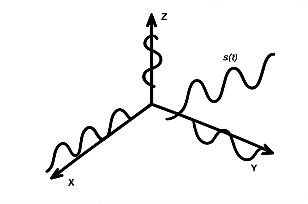
Orthogonal Decompositions
Building on our foundation: In our three previous articles (Signals as Vectors, L² Norms & Inner Product, Hilbert Spaces), we built the mathematical tools. Now we use them.
What we’ll actually do: Compute inner products. Lots of them.
Three types of inner products we’ll compute:
- ⟨s, φₖ⟩ — Signal with basis functions → extracts coefficients
- ⟨φₘ, φₙ⟩ — Basis function with basis function → verifies orthogonality
- ⟨φₖ, φₖ⟩ — Basis function with itself → finds norms for normalization
The basis functions φₖ: These are our chosen “building blocks”
- Fourier series (complex exponential version):
$$ \phi_k = e^{i 2\pi k t / T} $$
- Polynomial approximation: φₖ = Legendre polynomials
- Time-frequency analysis: φₖ = wavelets
Note: Not all wavelets are orthogonal. We will cover these topics separately
Why orthogonal decompositions work: The right basis functions make complex problems simple.
Inner products become our computational engine for real-world signal processing.
The Mathematical Trinity
When building any orthogonal decomposition system, three mathematical properties determine whether our basis will succeed or fail catastrophically:
Linear Independence: The Foundation of Uniqueness
The requirement: No basis function can be written as a combination of others.
Why it matters: Without linear independence, the same signal could be represented in multiple ways, leading to ambiguity and computational chaos. Imagine trying to navigate with a map where the same location could have different coordinates, mathematical disaster.
Mathematical test:
For a basis ${\phi_k}$, if $\sum c_k \phi_k = 0$, then all $c_k = 0$.
💡 Key Mathematical Insight: If a set of vectors is orthogonal, then linear independence is automatically guaranteed!
Proof: Suppose {φₖ} is orthogonal and ∑ cₖφₖ = 0. Taking the inner product with φₘ: ⟨∑ cₖφₖ, φₘ⟩ = ⟨0, φₘ⟩ = 0
By linearity: ∑ cₖ⟨φₖ, φₘ⟩ = 0
By orthogonality: only the k = m term survives, giving cₘ⟨φₘ, φₘ⟩ = 0
Since ⟨φₘ, φₘ⟩ ≠ 0 (non-zero vectors), we must have cₘ = 0 for all m.
This is why orthogonal bases are so powerful, they automatically satisfy the independence requirement while providing the computational advantages of orthogonality!
Orthogonality: The Gift of Simplicity
The requirement: Different basis functions have zero inner product.
Why it’s so cool : Orthogonality transforms the nightmare of solving coupled systems of equations into the dream of independent calculations. Each coefficient can be computed separately without interference from others.
Mathematical beauty:
⟨φₘ, φₙ⟩ = 0 for m ≠ n
Signals can be projected onto φₘ with L² norm cₘ as cₘ = ⟨s, φₘ⟩/⟨φₘ, φₘ⟩
Completeness: The Promise of Universality
The requirement: Every signal in our space can be represented using the basis.
Why it’s essential: Completeness guarantees that no signal “escapes” our representation. Without it, there would be signals that simply cannot be analyzed using our chosen basis, a fundamental limitation that dooms the entire approach.
Mathematical assurance: For any signal s, we can write s = ∑ cₖφₖ with arbitrary precision.
Fourier Series
Among all possible orthogonal decompositions, the Fourier series stands as the most elegant and widely applicable. It doesn’t just satisfy our trinity requirements, it does so with mathematical elegance that has made it the foundation of modern signal processing, communications, and countless other fields.
The Fourier series reveals that every periodic signal is secretly a sum of pure sinusoidal oscillations. This isn’t just a useful approximation, it’s a fundamental truth about the mathematical structure of periodic phenomena.
But the Fourier series is just one member of a vast family of orthogonal decompositions. Polynomial bases reveal smooth trends, wavelet bases capture transient phenomena, and custom orthogonal bases can be designed for specific applications. Each basis acts as a different lens, revealing different aspects of the same underlying signal.
Note: While the Fourier transform emerges as a limiting case when we let the period approach infinity, its rigorous treatment requires additional mathematical machinery involving measure theory and distribution theory. We’ll tackle that mathematical journey in a future exploration, building on the solid foundation we establish here with Fourier series.
Fourier Series: Trinity Test in Action
The Fourier series provides the gold standard example of our trinity principles. We’ll prove that complex exponentials don’t just work well, they’re mathematically optimal for frequency analysis.
The Choice: Sine/Cosine vs Complex Exponentials
👉 Here were are going to discuss a little bit of formal stuff. You can even skip this topic and comeback later.
For periodic signals with period T, we face a fundamental choice (if have gone through standard text books, you may have seen these two options in use.):
Option A — Traditional Trigonometric Basis:
$$ { 1, \cos\left(\frac{2\pi t}{T}\right), \sin\left(\frac{2\pi t}{T}\right), \cos\left(\frac{4\pi t}{T}\right), \sin\left(\frac{4\pi t}{T}\right), \cos\left(\frac{6\pi t}{T}\right), \sin\left(\frac{6\pi t}{T}\right), \ldots } $$
Option B — Complex Exponential Basis:
$$ { e^{\frac{-i4\pi t}{T}}, e^{\frac{-i2\pi t}{T}}, e^{i0}, e^{\frac{i2\pi t}{T}}, e^{\frac{i4\pi t}{T}}, \ldots } = { e^{\frac{i2\pi k t}{T}} \mid k = \ldots, -2, -1, 0, 1, 2, \ldots } $$
Euler’s Revelation: They’re the Same!
Here’s the mathematical magic, these aren’t different approaches, they’re identical:
$$ e^{\frac{i2\pi k t}{T}} = \cos\left(\frac{2\pi k t}{T}\right) + i \sin\left(\frac{2\pi k t}{T}\right) $$
What this means:
- Complex exponential is sine + cosine combined
- Not replacing trigonometric functions: unifying them
- One complex number = two real functions packaged together
The beautiful consequence:
- $e^{\frac{i2\pi t}{T}}$ contains both $\cos\left(\frac{2\pi t}{T}\right)$ and $\sin\left(\frac{2\pi t}{T}\right)$
- $e^{\frac{-i2\pi t}{T}}$ contains both $\cos\left(\frac{2\pi t}{T}\right)$ and $-\sin\left(\frac{2\pi t}{T}\right)$
- The full complex basis ${ e^{\frac{i2\pi k t}{T}} }$ contains all the trigonometric functions
Why choose the complex form?
- Unified mathematics: One elegant formula instead of separate sine/cosine cases
- Simpler algebra:
$$ e^{ia} \cdot e^{ib} = e^{i(a+b)} \quad \text{vs. trigonometric identities} $$
- Natural derivatives:
$$ \frac{d}{dt} \left[ e^{ikt} \right] = ik \cdot e^{ikt} $$
- Computational efficiency: Complex arithmetic is highly optimized
Trinity Test 1: Linear Independence
The complex exponentials {e^(i2πkt/T)} are linearly independent. To prove this, suppose:
$$ \sum_{k} c_k e^{\frac{i2\pi k t}{T}} = 0 \quad \text{for all } t $$
Taking the inner product with e^(-i2πkt/T) and using orthogonality (proven below), we get cₖ = 0 for all k. Therefore, the only solution is the trivial one, confirming linear independence.
Trinity Test 2: Orthogonality
Let’s compute the inner product of two complex exponentials over period T:
$$ \langle \phi_m, \phi_n \rangle = \int_0^T e^{\frac{i2\pi m t}{T}} \cdot \left[ e^{\frac{i2\pi n t}{T}} \right]^* dt $$
The conjugate gives us:
$$ \langle \phi_m, \phi_n \rangle = \int_0^T e^{\frac{i2\pi m t}{T}} \cdot e^{\frac{-i2\pi n t}{T}} , dt = \int_0^T e^{\frac{i2\pi (m - n) t}{T}} dt $$
Case 1: $m = n$
$$ \langle \phi_m, \phi_m \rangle = \int_0^T e^{i2\pi \cdot 0 \cdot t / T} dt = \int_0^T 1 dt = T $$
Case 2: $m \ne n$
$$ \langle \phi_m, \phi_n \rangle = \int_0^T e^{\frac{i2\pi (m - n) t}{T}} dt = \left[ \frac{T}{i2\pi (m - n)} e^{\frac{i2\pi (m - n) t}{T}} \right]_0^T $$
$$ = \frac{T}{i2\pi (m - n)} \left[ e^{i2\pi (m - n)} - 1 \right] = \frac{T}{i2\pi (m - n)} [1 - 1] = 0 $$
Perfect orthogonality! The basis functions are orthogonal but not orthonormal.
Finding the L² Norm and Unit Vectors:
The L² norm of each basis function is:
$$ | \phi_k |_2 = \sqrt{ \langle \phi_k, \phi_k \rangle } = \sqrt{T} $$
To create an orthonormal basis, we normalize:
$$ \psi_k(t) = \frac{1}{\sqrt{T}} e^{\frac{i2\pi k t}{T}} $$
Now the orthonormality condition becomes: ⟨ψₘ, ψₙ⟩ = δₘₙ
where δₘₙ is the Kronecker delta.
Trinity Test 3: Completeness
The complex exponential basis is complete in L²[0,T]. This means that for any square-integrable periodic function s(t), we can write:
$$ s(t) = \sum_{k=-\infty}^{\infty} c_k e^{\frac{i2\pi k t}{T}} $$
The series converges in the L² sense. The completeness property ensures that the Fourier series representation can capture any periodic signal with finite energy, making it universally applicable for signal analysis.
Note on completeness proofs: The rigorous proof of completeness for complex exponentials and trigonometric series involves advanced techniques from functional analysis and is beyond the scope of this blog. We focus here on the computational and conceptual aspects that make these bases so powerful in practice.
Computing Fourier Coefficients via Inner Product
With our orthonormal basis,
$$ \psi_k(t) = \frac{1}{\sqrt{T}} e^{\frac{i2\pi k t}{T}} $$
The coefficients are:
$$ c_k = \langle s, \psi_k \rangle = \int_0^T s(t) \cdot [\psi_k(t)]^* dt $$
Substituting our basis:
$$ c_k = \int_0^T s(t) \cdot \left[ \frac{1}{\sqrt{T}} e^{\frac{i2\pi k t}{T}} \right]^* dt = \frac{1}{\sqrt{T}} \int_0^T s(t) \cdot e^{\frac{-i2\pi k t}{T}} dt $$
Did you see? The negative sign in the complex exponential came from conjugation. That’s how we “had to” define our inner product in order to comply with the inner product’s rules (Check my previous post on the topic).
From Series to Transform: A Mathematical Bridge
The Fourier series provides the foundation for understanding frequency analysis of periodic signals. The continuous Fourier transform emerges as a limiting case when we let the period T → ∞, but this limiting process requires careful mathematical treatment involving measure theory and distribution theory.
This limiting transition is profound; we move from a discrete spectrum (countable frequencies) to a continuous spectrum (uncountable frequencies). While conceptually elegant, the rigorous mathematical treatment deserves its own dedicated exploration where we can properly address convergence issues, generalized functions, and the measure-theoretic foundations.
For now, we focus on mastering the Fourier series, which provides all the essential insights about frequency analysis while remaining mathematically concrete and rigorous.
Why Fourier Works So Well
The complex exponential basis functions are eigenfunctions of the differentiation operator:
$$ \frac{d}{dt} \left[ e^{ikt} \right] = ik \cdot e^{ikt} $$
This eigenfunction property means:
- Derivatives become multiplication by iω in frequency domain
- Convolution becomes multiplication
- Linear time-invariant systems become simple multiplication
This is why Fourier analysis is so powerful for linear systems, it transforms differential equations into algebraic ones.
Beyond Fourier: The Polynomial Perspective
The Surprising Truth: Polynomials Can Be Orthogonal
At first glance, polynomials like 1, x, x², x³, … seem to have nothing to do with orthogonality. After all, these simple monomials are clearly not orthogonal to each other under the standard L² inner product. But here’s the mathematical surprise: there exist polynomials that are orthogonal!
The key insight is that orthogonality depends on three things:
- The interval we’re working on
- The weight function we use in the inner product
- The specific polynomials we choose
By carefully selecting these elements, mathematicians have discovered families of polynomials that satisfy our trinity requirements perfectly. These orthogonal polynomials form the foundation for polynomial-based signal analysis, numerical approximation, and mathematical physics.
The orthogonal polynomial families include:
- Legendre polynomials: Orthogonal on [-1,1] with uniform weight
- Chebyshev polynomials: Orthogonal on [-1,1] with weight 1/√(1-x²)
- Hermite polynomials: Orthogonal on (-∞,∞) with Gaussian weight e^(-x²)
- Laguerre polynomials: Orthogonal on [0,∞) with exponential weight e^(-x)
Each family is tailored for specific applications, but all share the beautiful property that different polynomials in the family are orthogonal to each other under their respective weighted inner products.
Legendre Polynomials: Orthogonality on [-1,1]
The Legendre polynomials {P₀(x), P₁(x), P₂(x), …} form an orthogonal basis on [-1,1] with the standard inner product:
- $P_0(x) = 1$
- $P_1(x) = x$
- $P_2(x) = \frac{3x^2 - 1}{2}$
- $P_3(x) = \frac{5x^3 - 3x}{2}$
- $\ldots$
They satisfy the orthogonality condition:
$$ \int_{-1}^1 P_m(x) P_n(x) dx = \frac{2}{2n + 1} \delta_{mn} $$
Applications: Legendre polynomials excel at approximating smooth functions and are widely used in numerical analysis and physics (spherical harmonics are built from them).
Chebyshev Polynomials: Minimax Optimization
Chebyshev polynomials of the first kind are defined by: Tₙ(cos θ) = cos(nθ)
They’re orthogonal with respect to the weight function 1/√(1-x²):

The minimax property: Among all monic polynomials of degree n, the Chebyshev polynomial (scaled) has the smallest maximum absolute value on [-1,1]. This makes Chebyshev polynomials optimal for polynomial approximation in the uniform norm.
Hermite Polynomials: Gaussian Weight
Hermite polynomials are orthogonal with respect to the Gaussian weight e^(-x²):

They appear naturally in quantum mechanics (These arise as solutions to the Schrödinger equation for the quantum harmonic oscillator, and their properties, such as orthogonality, are crucial for understanding the quantum behavior of oscillating particles.) and in the analysis of Gaussian processes.
Wavelets: Time-Frequency Localization
While Fourier analysis gives perfect frequency resolution, it has no time localization. Wavelets provide a basis that’s localized in both time and frequency.
The Wavelet Transform
A wavelet basis is generated by translations and dilations of a mother wavelet ψ(t):
$$ \psi_{a,b}(t) = \frac{1}{\sqrt{a}} \psi \left( \frac{t - b}{a} \right) $$
where a controls scale (frequency) and b controls translation (time).
Orthogonality: Properly chosen wavelets form orthogonal bases, allowing efficient computation while maintaining time-frequency localization. Not all wavelet types are orthogonal (We will cover in a separate article)
Completeness: Wavelet bases are complete for L², meaning any finite-energy signal can be perfectly reconstructed.
Choosing Your Basis: A Practical Guide
For Periodic Signals or Frequency Analysis
- Fourier series/transform: Unmatched for linear system analysis, filtering, and spectral analysis
- Discrete Fourier Transform (DFT): Computationally efficient via FFT
For Smooth, Non-Periodic Functions
- Legendre polynomials: Excellent for smooth approximation on bounded intervals
- Chebyshev polynomials: Optimal for minimax approximation
- Power series: Simple but convergence can be limited
For Transient or Localized Phenomena
- Wavelets: Superior for signals with both time and frequency structure
- Gabor functions: Gaussian-windowed sinusoids for time-frequency analysis
For Data with Specific Statistical Properties
- Hermite polynomials: Natural for Gaussian processes
- Laguerre polynomials: Useful for exponentially decaying signals
The Deeper Truth: Bases Reveal Hidden Structure
Each basis acts as a lens, revealing different aspects of signals:
- Fourier basis: Reveals periodic structure and frequency content
- Polynomial bases: Capture smooth variations and global trends
- Wavelet bases: Expose transient events and multi-scale structure
- Empirical bases (like Principal Components): Reveal the most important variations in data
The choice of basis isn’t just mathematical convenience; it’s about matching the basis to the underlying structure of your signals. A speech signal might be best analyzed with wavelets to capture both phonetic content (frequency) and timing. A slowly varying sensor measurement might be perfectly captured with a few Legendre polynomial coefficients.
Conclusion
Each orthogonal basis reveals different signal structure: Fourier exposes frequencies, polynomials capture smooth trends, wavelets reveal transients. The trinity, independence, orthogonality, completeness makes them all work.
Fourier series achieves mathematical perfection in satisfying these requirements, unifying trigonometric functions into complex exponentials and forming the foundation of modern signal processing.
A big piece of signal processing is about decomposition, finding the right way to break signals apart that reveals their essential structure.
Next: We’ll see how AM radio receivers work as inner products in action, the mathematics of tuning into your favorite station.