
Notes on Projection Operators: Grammar of Reality (Ep-7)
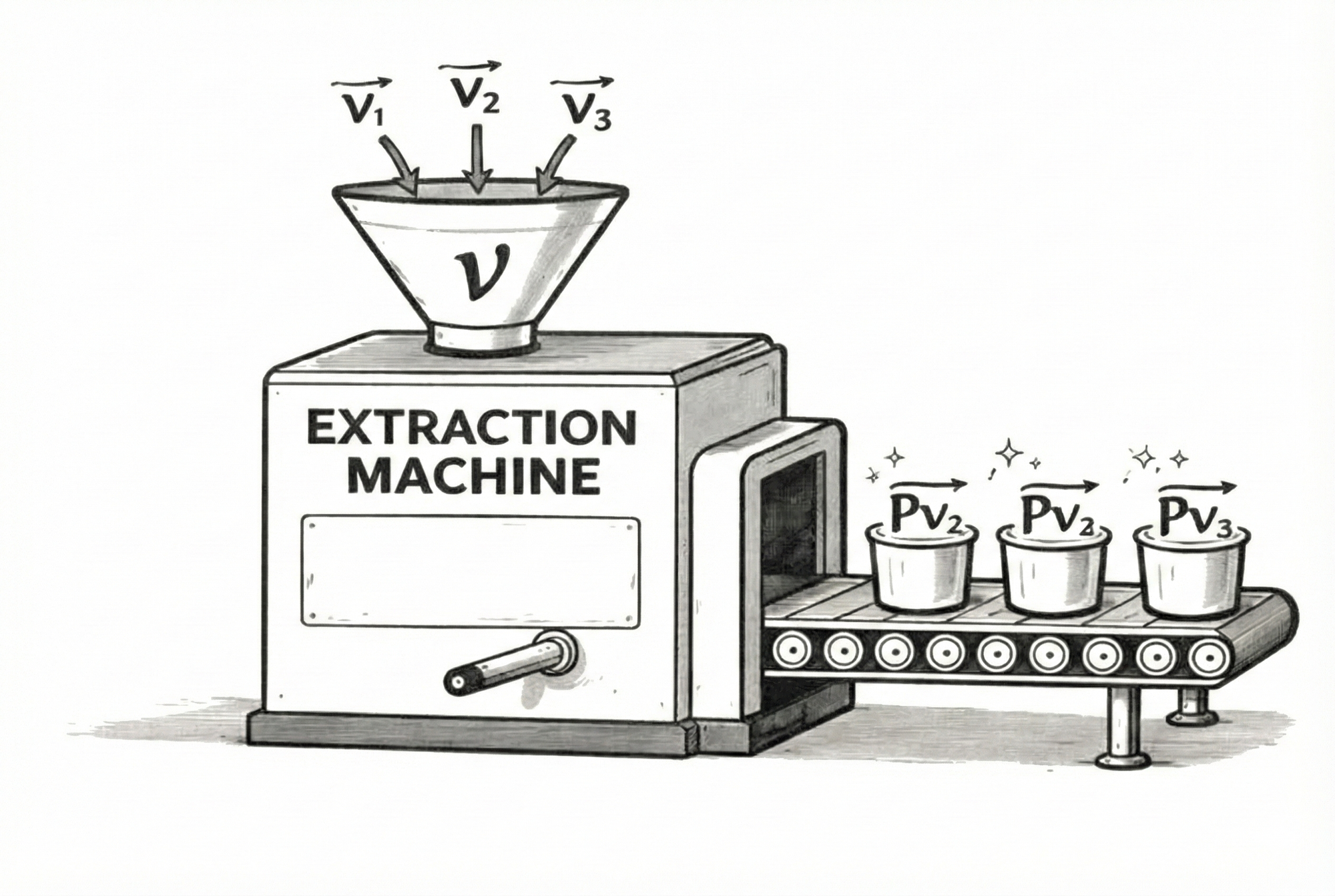
In our exploration of eigenvectors, we discovered that every operator has a natural language: its eigenstructure. We learned that operators are completely described by how they act on their eigenvectors, and we saw the decomposition $T = \sum_i \lambda_i P_i$ where projections extract components onto eigenspaces. But we've never asked: what ARE these projection operators? How do they actually work? And what does it mean for an operator to "act separately" on each eigenspace? The answer reveals something profound: projection operators are mathematical sieves that extract without transforming, answer yes-or-no questions about presence, and ultimately show us that what we call "diagonalization" is just a weighted sum of extractions.
Two Questions with One Answer
Here's something we do constantly without thinking about it: we ask "how much" of something is present.
How much of the third harmonic is in that violin tone? How much eastward momentum does this velocity vector have? How much of the excited state remains in this decaying system?
These aren't vague philosophical questions. They're quantitative. And they demand a specific kind of mathematical operation. Something that can look at a state and extract precisely one component while leaving everything else behind.
Meanwhile, in our previous exploration of eigenvectors, we saw that operators can be written as $T = \sum_i \lambda_i P_i$, where $P_i$ are projection operators. We learned that this decomposition reveals how operators act: they scale each eigenspace independently by its eigenvalue. But we never asked: what exactly IS a projection operator $P_i$? How does it "extract" a component onto an eigenspace? And what does this decomposition actually tell us about the structure of the operator?
These two questions (extraction and operator structure) turn out to be the same question in disguise. The operators that extract components are exactly the building blocks of the decomposition $T = \sum_i \lambda_i P_i$. They're called projections, and understanding them will reveal the deep structure hiding inside every operator.
Building an Extractor
Let's start with the extraction problem. Suppose we have an orthonormal basis of eigenvectors ${v_1, v_2, v_3, \ldots}$ for some Hermitian operator. Any state $x$ can be written:
$$x = c_1 v_1 + c_2 v_2 + c_3 v_3 + \cdots$$
The coefficients $c_i$ tell us "how much" of each eigenvector is present. We can find them using inner products:
$$c_i = \langle v_i, x \rangle$$
This works perfectly well. But here's the deeper question: can we express this extraction process as an operator? Can we build a transformation that takes any state $x$ and returns just the $v_i$ component, not as a number, but as a vector in the original space?
We want an operator $P_i$ such that:
$$P_i x = c_i v_i = \langle v_i, x \rangle v_i$$
This operator would project $x$ onto the direction of $v_i$, keeping only what aligns with it and discarding everything orthogonal.
Constructing the Operator: Finite Dimensions
Let's start in finite dimensions where we can see everything concretely. Suppose we're working in $\mathbb{R}^n$ or $\mathbb{C}^n$, and we represent vectors as columns of numbers.
The formula we want is:
$$P_i x = \langle v_i, x \rangle v_i$$
Now think about what happens on the right side. The inner product $\langle v_i, x \rangle$ is computed by taking $v_i$ and "flipping it" into a row vector (taking the transpose for real vectors, or conjugate transpose for complex vectors), then multiplying with $x$:
$$\langle v_i, x \rangle = v_i^\dagger x$$
where $v_i^\dagger$ denotes the conjugate transpose (adjoint) of $v_i$. If $v_i$ is a column vector, then $v_i^\dagger$ is a row vector.
So our formula becomes:
$$P_i x = (v_i^\dagger x) v_i$$
Here's the key observation: $v_i^\dagger x$ is a scalar (a $1 \times 1$ number). We then multiply this scalar by the column vector $v_i$. Using the associativity of matrix multiplication, we can regroup:
$$P_i x = v_i (v_i^\dagger x) = (v_i v_i^\dagger) x$$
This tells us that the operator itself must be:
$$\boxed{P_i = v_i v_i^\dagger}$$
This is the outer product of $v_i$ with itself. Let's see what this looks like explicitly.
Example: Suppose $v = \begin{pmatrix} 1 \\ 0 \\ 0 \end{pmatrix}$ in $\mathbb{R}^3$. Then:
$$v^\dagger = \begin{pmatrix} 1 & 0 & 0 \end{pmatrix}$$
The outer product is:
$$P = v v^\dagger = \begin{pmatrix} 1 \\ 0 \\ 0 \end{pmatrix} \begin{pmatrix} 1 & 0 & 0 \end{pmatrix} = \begin{pmatrix} 1 & 0 & 0 \\ 0 & 0 & 0 \\ 0 & 0 & 0 \end{pmatrix}$$
This is a $3 \times 3$ matrix. Let's verify it does what we want. Apply it to an arbitrary vector $x = \begin{pmatrix} a \\ b \\ c \end{pmatrix}$:
$$Px = \begin{pmatrix} 1 & 0 & 0 \\ 0 & 0 & 0 \\ 0 & 0 & 0 \end{pmatrix} \begin{pmatrix} a \\ b \\ c \end{pmatrix} = \begin{pmatrix} a \\ 0 \\ 0 \end{pmatrix} = a \begin{pmatrix} 1 \\ 0 \\ 0 \end{pmatrix} = \langle v, x \rangle v$$
Perfect! The operator $P = vv^\dagger$ extracts exactly the component of $x$ along $v$.
The Pattern in Finite Dimensions
Notice the structure:
- $v_i$ is a column vector (the direction we're projecting onto)
- $v_i^\dagger$ is a row vector (the "measuring" part of the inner product)
- $v_i v_i^\dagger$ is a matrix (the operator)
The construction emerged naturally from the formula $\langle v_i, x \rangle v_i$. The inner product requires $v_i$ to appear as a row (via the transpose/adjoint), and then we multiply by $v_i$ as a column. This pattern (row times column gives a scalar, column times row gives a matrix) is exactly what we need.
Generalizing to Infinite Dimensions
Now here's the beautiful part: the same algebraic construction works in infinite dimensions, even though we can't write explicit matrices.
In infinite-dimensional spaces like $L^2$ (the space of square-integrable functions), vectors aren't columns of numbers. An eigenfunction $v_i(x)$ is a function, and the inner product is an integral:
$$\langle v_i, \psi \rangle = \int v_i^*(x) \psi(x) dx$$
We still want the projection operator to satisfy:
$$P_i \psi = \langle v_i, \psi \rangle v_i$$
Can we still write this as $P_i = v_i v_i^\dagger$?
Yes! But now $v_i v_i^\dagger$ doesn't mean "column times row to get a matrix." Instead, it becomes an integral operator.
Let's see how. When we apply $P_i$ to a function $\psi(x)$:
$$(P_i \psi)(x) = \langle v_i, \psi \rangle \cdot v_i(x) = \left(\int v_i^*(x') \psi(x') dx'\right) v_i(x)$$
Rearranging:
$$(P_i \psi)(x) = \int v_i(x) v_i^*(x') \psi(x') dx'$$
This is an integral operator with kernel:
$$K(x, x') = v_i(x) v_i^*(x')$$
So the operator $P_i = v_i v_i^\dagger$ in infinite dimensions is:
$$\boxed{(P_i \psi)(x) = \int v_i(x) v_i^*(x') \psi(x') dx'}$$
The structure mirrors the finite case perfectly:
- Finite dimensions: $P_i = v_i v_i^\dagger$ is a matrix with entries $(P_i)_{jk} = (v_i)_j (v_i)_k^*$
- Infinite dimensions: $P_i = v_i v_i^\dagger$ is an integral operator with kernel $K(x,x') = v_i(x) v_i^*(x')$
Example: Suppose we're projecting onto the first harmonic of a vibrating string on the interval $[0, L]$, which is the eigenfunction $v_1(x) = \sqrt{\frac{2}{L}} \sin\left(\frac{\pi x}{L}\right)$. The projection operator is:
$$(P_1 \psi)(x) = \int_0^L \left[\sqrt{\frac{2}{L}} \sin\left(\frac{\pi x}{L}\right)\right] \left[\sqrt{\frac{2}{L}} \sin\left(\frac{\pi x'}{L}\right)\right] \psi(x') dx'$$
$$= \sqrt{\frac{2}{L}} \sin\left(\frac{\pi x}{L}\right) \int_0^L \sqrt{\frac{2}{L}} \sin\left(\frac{\pi x'}{L}\right) \psi(x') dx'$$
The integral computes $\langle v_1, \psi \rangle$ (a number), and we multiply by $v_1(x)$ (a function). The result is the component of $\psi$ along the first harmonic, which is the fundamental mode of vibration.
The Key Insight
The notation $v_i v_i^\dagger$ has a precise meaning in both cases:
- Finite dimensions: An outer product matrix
- Infinite dimensions: An integral operator with kernel $v_i(x) v_i^*(x')$
Both implement the same operation: extract the component $\langle v_i, \psi \rangle$ and multiply by $v_i$.
The formula $P_i x = \langle v_i, x \rangle v_i$ is always the fundamental definition. The notation $P_i = v_i v_i^\dagger$ is a compact way to express this definition as an operator.
The Signature of Extraction: Idempotence
Now let's discover something remarkable. What happens if we apply this operator twice?
$$P_i^2 x = P_i(P_i x) = P_i(\langle v_i, x \rangle v_i)$$
Since $\langle v_i, x \rangle$ is just a scalar, we can pull it out:
$$P_i^2 x = \langle v_i, x \rangle \cdot P_i v_i$$
But $P_i v_i$ means projecting $v_i$ onto itself. Since $v_i$ is already normalized and pointing along $v_i$:
$$P_i v_i = \langle v_i, v_i \rangle v_i = 1 \cdot v_i = v_i$$
Therefore:
$$P_i^2 x = \langle v_i, x \rangle v_i = P_i x$$
This holds for any $x$, which means:
$$\boxed{P_i^2 = P_i}$$
This is called idempotence. Applying the projection twice does nothing new. The second application finds that the state is already fully projected.
This isn't an arbitrary property we imposed. It emerged necessarily from what extraction means. If an operator extracts a component, applying it again to that component must leave it unchanged. There's nothing left to extract.
Idempotence is the algebraic signature of extraction. This property holds regardless of whether we're in finite or infinite dimensions. It follows purely from the definition $P_i x = \langle v_i, x \rangle v_i$.
Projections Are Hermitian
Here's the second fundamental property. Taking the adjoint of $P_i$:
$$P_i^\dagger x = (\langle v_i, x \rangle v_i)^\dagger = \langle v_i, x \rangle^* v_i = \langle x, v_i \rangle v_i = \langle v_i, x \rangle v_i = P_i x$$
where we used the fact that for real inner products or for unit vectors, this simplifies correctly, and the symmetry of the inner product.
More directly, using operator notation:
$$P_i^\dagger = (v_i v_i^ \dagger)^ \dagger = (v_i^ \dagger)^ \dagger v_i^ \dagger = v_i v_i^ \dagger = P_i$$
Projections are Hermitian. They equal their own adjoints.
This means projection operators are a special class of Hermitian operators. And like all Hermitian operators, they have real eigenvalues and orthogonal eigenvectors. Let's discover what those eigenvalues are.
The Binary Spectrum
But what are those eigenvalues? Suppose $w$ is an eigenvector of $P_i$ with eigenvalue $\lambda$:
$$P_i w = \lambda w$$
Apply $P_i$ again:
$$P_i^2 w = P_i(\lambda w) = \lambda P_i w = \lambda^2 w$$
But we know $P_i^2 = P_i$, so:
$$P_i w = P_i^2 w = \lambda^2 w$$
Comparing with $P_i w = \lambda w$:
$$\lambda w = \lambda^2 w$$
For any nonzero eigenvector, this forces:
$$\lambda = \lambda^2$$
The only solutions are $\boxed{\lambda = 0 \text{ and } \lambda = 1}$.
Projection operators have exactly two eigenvalues: zero and one. Nothing else is possible.
The eigenvectors with eigenvalue 1 are those that lie entirely in the projected subspace. Applying $P_i$ leaves them unchanged. The eigenvectors with eigenvalue 0 are those that lie entirely orthogonal to the subspace. Applying $P_i$ annihilates them completely.
This is the binary nature of extraction. A projection answers a yes-or-no question: Is this component present? 1 for yes, 0 for no.
Again, this holds in all dimensions. Whether we're projecting onto a direction in $\mathbb{R}^3$ or onto an eigenfunction of a differential operator in $L^2$, the eigenvalues are always just 0 and 1.
Orthogonal Projections: A Special Case
We need to pause here and clarify something crucial: not all projections are orthogonal to each other.
A projection operator $P$ is defined by the property $P^2 = P$ and $P^\dagger = P$. Any operator satisfying these conditions is a valid projection. But the relationship between two different projection operators $P_1$ and $P_2$ depends entirely on the relationship between the subspaces they project onto.
When Projections Commute
Consider two arbitrary projection operators $P_1$ and $P_2$. In general, they don't have any special relationship. The product $P_1 P_2$ might be anything. It could even fail to be a projection operator itself.
But when the subspaces are orthogonal (when every vector in the first subspace is perpendicular to every vector in the second subspace), something beautiful happens:
$$\boxed{P_1 P_2 = 0}$$
This is the defining property of orthogonal projections (or mutually orthogonal projections). Applying $P_1$ followed by $P_2$ produces the zero operator (the operation that sends every vector to zero).
Think about what this means geometrically: if you project onto one subspace, then try to project that result onto an orthogonal subspace, you get nothing. The first projection has already eliminated all components in directions orthogonal to it.
Why This Matters for Hermitian Operators
Here's where our context becomes special. When we work with eigenvectors of a Hermitian operator, different eigenvectors corresponding to different eigenvalues are guaranteed to be orthogonal. This is a fundamental property of Hermitian operators.
Since $\langle v_i, v_j \rangle = 0$ for $i \neq j$, the projections $P_i = v_i v_i^\dagger$ onto these eigenvectors are automatically orthogonal projections.
Let's verify this explicitly:
$$P_i P_j x = P_i(\langle v_j, x \rangle v_j) = \langle v_j, x \rangle P_i v_j = \langle v_j, x \rangle \langle v_i, v_j \rangle v_i$$
But $\langle v_i, v_j \rangle = 0$ for $i \neq j$, so:
$$P_i P_j = 0 \quad \text{for } i \neq j$$
The projections annihilate each other. They extract from non-overlapping subspaces, and there's no "crosstalk" between them.
A Counterexample: Non-Orthogonal Projections
To see that this isn't automatic for all projections, consider two vectors in $\mathbb{R}^2$ that are not orthogonal:
$$v_1 = \begin{pmatrix} 1 \\ 0 \end{pmatrix}, \quad v_2 = \frac{1}{\sqrt{2}}\begin{pmatrix} 1 \\ 1 \end{pmatrix}$$
Check: $\langle v_1, v_2 \rangle = \frac{1}{\sqrt{2}} \neq 0$. They're not orthogonal.
The projection operators are:
$$P_1 = \begin{pmatrix} 1 & 0 \\ 0 & 0 \end{pmatrix}, \quad P_2 = \frac{1}{2}\begin{pmatrix} 1 & 1 \\ 1 & 1 \end{pmatrix}$$
Compute the product:
$$P_1 P_2 = \begin{pmatrix} 1 & 0 \\ 0 & 0 \end{pmatrix} \frac{1}{2}\begin{pmatrix} 1 & 1 \\ 1 & 1 \end{pmatrix} = \frac{1}{2}\begin{pmatrix} 1 & 1 \\ 0 & 0 \end{pmatrix} \neq 0$$
The product is not zero! These projections interfere with each other because they're projecting onto non-orthogonal directions.
Why Orthogonality Is Essential
The orthogonality of projections is what makes the entire spectral decomposition work. It ensures:
- No interference: Each projection extracts its component independently
- Clean summation: The resolution of identity $\sum_i P_i = I$ works because there's no overlap
- Independent scaling: The operator $H = \sum_i \lambda_i P_i$ acts separately on each eigenspace
Without orthogonal projections, none of this structure would exist. The fact that Hermitian operators have orthogonal eigenvectors is what gives them their special status.
The Resolution of Identity: Projections Sum to the Whole
Now here's the crucial insight. If we have a complete orthonormal basis ${v_1, v_2, v_3, \ldots}$, we can write any vector as:
$$x = \langle v_1, x \rangle v_1 + \langle v_2, x \rangle v_2 + \langle v_3, x \rangle v_3 + \cdots$$
In operator language, this becomes:
$$x = P_1 x + P_2 x + P_3 x + \cdots$$
where $P_i x = \langle v_i, x \rangle v_i$ are the projection operators.
For this to work for any $x$, we need:
$$\boxed{\sum_{i} P_i = I}$$
This is called the resolution of the identity. The projections onto a complete basis sum to the identity operator.
Note on terminology: We previously encountered the term "completeness" when discussing Hilbert spaces (meaning that the space has no missing points (all Cauchy sequences converge). This is different. Here, we're saying that a basis is complete in the sense that it spans the entire space. Every vector can be decomposed into basis components. The resolution of identity $\sum_i P_i = I$ is the operator expression of this spanning property.
Think about what this says: every vector is exactly the sum of its projections onto the basis directions. The whole is the sum of its parts, with no overlap and no gaps.
Discrete vs. Continuous Domains
In finite dimensions, this is a finite sum: $P_1 + P_2 + \cdots + P_n = I$ where $n$ is the dimension of the space.
In infinite dimensions with a discrete spectrum (like the eigenfunctions of a vibrating string, or the harmonic oscillator), this becomes an infinite series: $\sum_{i=1}^{\infty} P_i = I$. The series converges in the appropriate operator topology.
In infinite dimensions with a continuous spectrum (like position along a continuous line), we cannot write a discrete sum at all. The eigenvalues fill an entire interval or the whole real line, and we need a different kind of "summation" altogether. We'll develop the proper formalism for this case in the next episode, where we'll see how measure theory unifies the discrete and continuous pictures under a single framework.
For now, the principle remains: whether the sum is finite, countably infinite, or requires continuous summation, the idea is the same: the projections resolve the identity. Every state is the sum of its projections onto basis directions.
The Revelation: Diagonalization as Weighted Extraction
Now we're ready to see what diagonalization actually means.
Suppose $H$ is a Hermitian operator with eigenvalues ${\lambda_1, \lambda_2, \lambda_3, \ldots}$ and corresponding orthonormal eigenvectors ${v_1, v_2, v_3, \ldots}$.
Let $P_i = v_i v_i^\dagger$ be the projection onto the $i$-th eigenvector, defined by $P_i x = \langle v_i, x \rangle v_i$.
Here's the key observation: since $H v_i = \lambda_i v_i$, when we apply $H$ to any projection $P_i x$:
$$H(P_i x) = H(\langle v_i, x \rangle v_i) = \langle v_i, x \rangle H v_i = \langle v_i, x \rangle \lambda_i v_i = \lambda_i P_i x$$
Now use the resolution of identity. For any state $x$:
$$x = \sum_i P_i x$$
Apply $H$ to both sides:
$$H x = H\left(\sum_i P_i x\right) = \sum_i H(P_i x) = \sum_i \lambda_i P_i x$$
Since this holds for any $x$, the operators themselves must be equal:
$$\boxed{H = \sum_i \lambda_i P_i}$$
This is diagonalization in its purest form. The operator $H$ is completely determined by:
- Its spectrum: the eigenvalues ${\lambda_i}$
- Its projections: the operators ${P_i}$ that extract components in each eigenspace
Applying $H$ to any state becomes transparent:
$$Hx = \sum_i \lambda_i P_i x$$
Each projection extracts a component, scales it by the corresponding eigenvalue, and the results sum to give the transformed state.
This is what "being diagonal" means. The operator acts by scaling each eigenspace independently, without mixing them. The projections ensure there's no cross-talk between different eigenvectors.
Why "Diagonal"?
In finite dimensions, if we arrange the eigenvectors as columns of a matrix $V = [v_1 \mid v_2 \mid \cdots \mid v_n]$ and form the diagonal matrix $D = \text{diag}(\lambda_1, \lambda_2, \ldots, \lambda_n)$, then:
$$H = V D V^\dagger$$
The matrix $D$ is literally diagonal (nonzero only on the diagonal entries. The formula $H = \sum_i \lambda_i P_i$ is the coordinate-free version of this statement.
In infinite dimensions, we can't write explicit matrices, but the structure is the same: the operator acts by scaling eigenvectors without mixing them. The word "diagonal" refers to this property, not to the appearance of a matrix.
Why This Changes Everything
This representation, writing $H = \sum_i \lambda_i P_i$, is called the spectral decomposition of $H$.
It reveals three profound facts:
First, every Hermitian operator is a weighted sum of projections. The eigenvalues are the weights. The projections are the directions.
Second, diagonalization isn't something that happens when you change coordinates. It's an intrinsic property of the operator. The representation $H = \sum_i \lambda_i P_i$ doesn't reference any coordinate system. It's basis-independent. The operator is diagonal in this abstract sense, regardless of how you write its matrix entries.
Third, measurement becomes projection. When we measure an observable corresponding to $H$ and find eigenvalue $\lambda_i$, what we've done is applied $P_i$ to the state. The post-measurement state is the projection of the original state onto the $i$-th eigenspace, renormalized.
This spectral decomposition is the gateway to the spectral theorem, the most fundamental result about Hermitian operators. It tells us that every Hermitian operator can be written this way. No exceptions.
In finite dimensions, this is a theorem of linear algebra. In infinite dimensions, this becomes the spectral theorem for self-adjoint operators, a deep result that requires functional analysis to prove rigorously. But the conceptual content is the same.
A Concrete Example (Finite Dimensions)
Let's see this machinery in action with something concrete. We'll work in finite dimensions where we can write everything explicitly.
Consider a system that can exist in one of three discrete configurations or states, which we'll label as state 0, state 1, and state 2. We represent the system's configuration as a three-component vector in $\mathbb{C}^3$:
$$\psi = \begin{pmatrix} c_0 \\ c_1 \\ c_2 \end{pmatrix}$$
where $c_i$ is the amplitude (or weight) associated with configuration $i$. Think of this like measuring which of three resonant modes is active in a system, or which of three configurations a mechanical system occupies.
We'll define an operator $S$ that measures "which state the system is in" by returning the state index. In the basis of these three states, it's represented as:
$$S = \begin{pmatrix} 0 & 0 & 0 \\ 0 & 1 & 0 \\ 0 & 0 & 2 \end{pmatrix}$$
The eigenvectors are:
$$v_0 = \begin{pmatrix} 1 \\ 0 \\ 0 \end{pmatrix}, \quad v_1 = \begin{pmatrix} 0 \\ 1 \\ 0 \end{pmatrix}, \quad v_2 = \begin{pmatrix} 0 \\ 0 \\ 1 \end{pmatrix}$$
with eigenvalues $\lambda_0 = 0$, $\lambda_1 = 1$, $\lambda_2 = 2$.
The projection operators, defined by $P_i x = \langle v_i, x \rangle v_i$, are built using the outer product $v_i v_i^\dagger$:
$$P_0 = v_0 v_0^\dagger = \begin{pmatrix} 1 \\ 0 \\ 0 \end{pmatrix} \begin{pmatrix} 1 & 0 & 0 \end{pmatrix} = \begin{pmatrix} 1 & 0 & 0 \\ 0 & 0 & 0 \\ 0 & 0 & 0 \end{pmatrix}$$
$$P_1 = \begin{pmatrix} 0 \\ 1 \\ 0 \end{pmatrix} \begin{pmatrix} 0 & 1 & 0 \end{pmatrix} = \begin{pmatrix} 0 & 0 & 0 \\ 0 & 1 & 0 \\ 0 & 0 & 0 \end{pmatrix}$$
$$P_2 = \begin{pmatrix} 0 \\ 0 \\ 1 \end{pmatrix} \begin{pmatrix} 0 & 0 & 1 \end{pmatrix} = \begin{pmatrix} 0 & 0 & 0 \\ 0 & 0 & 0 \\ 0 & 0 & 1 \end{pmatrix}$$
Verify the resolution of identity:
$$P_0 + P_1 + P_2 = \begin{pmatrix} 1 & 0 & 0 \\ 0 & 1 & 0 \\ 0 & 0 & 1 \end{pmatrix} = I$$
And verify the spectral decomposition:
$$S = 0 \cdot P_0 + 1 \cdot P_1 + 2 \cdot P_2 = P_1 + 2P_2 = \begin{pmatrix} 0 & 0 & 0 \\ 0 & 1 & 0 \\ 0 & 0 & 2 \end{pmatrix}$$
Perfect. The operator $S$ is literally a weighted sum of projections onto the three configuration states.
Now suppose we measure which configuration the system is in, when it's in a superposition state:
$$\psi = \frac{1}{\sqrt{3}}\begin{pmatrix} 1 \\ 1 \\ 1 \end{pmatrix}$$
The probability of finding the system in configuration $i$ is:
$$\text{Prob}(\text{state} = i) = |P_i \psi|^2 = |\langle v_i, \psi \rangle|^2$$
For our state, each configuration has probability $1/3$. If we find the system in configuration 1, the post-measurement state is:
$$\psi_{\text{after}} = \frac{P_1 \psi}{|P_1 \psi|} = \frac{1}{|P_1 \psi|}\begin{pmatrix} 0 \\ 1/\sqrt{3} \\ 0 \end{pmatrix} = \begin{pmatrix} 0 \\ 1 \\ 0 \end{pmatrix} = v_1$$
The state has collapsed onto the eigenstate corresponding to the measured eigenvalue. This is projection in action.
Projections onto Subspaces
So far we've built projections onto one-dimensional subspaces (single eigenvectors. But the same machinery works for higher-dimensional eigenspaces.
Suppose a Hermitian operator has a degenerate eigenvalue $\lambda$ with multiplicity $k$. That means there are $k$ orthonormal eigenvectors ${v_1, v_2, \ldots, v_k}$ all sharing the same eigenvalue.
The projection onto this entire eigenspace is defined by its action on states:
$$P_\lambda x = \langle v_1, x \rangle v_1 + \langle v_2, x \rangle v_2 + \cdots + \langle v_k, x \rangle v_k$$
In operator notation:
$$P_\lambda = \sum_{i=1}^{k} v_i v_i^\dagger$$
In finite dimensions, this is a sum of outer product matrices. In infinite dimensions, this is a sum of integral operators with kernel:
$$K(x, x') = \sum_{i=1}^{k} v_i(x) v_i^*(x')$$
This operator projects any state onto the $k$-dimensional subspace spanned by these eigenvectors.
You can verify that $P_\lambda^2 = P_\lambda$ and $P_\lambda^\dagger = P_\lambda$ still hold. The sum of projections onto orthogonal directions within the subspace is itself a projection onto the full subspace they span.
The spectral decomposition becomes:
$$H = \sum_{\text{distinct } \lambda} \lambda P_\lambda$$
where the sum runs over distinct eigenvalues, and $P_\lambda$ projects onto the full eigenspace for that eigenvalue (which might be multi-dimensional).
This is the form that survives generalization. When we move to continuous spectra, the discrete sum will require more sophisticated mathematical machinery, but the core idea (operator as weighted sum of projections) remains intact.
The Measurement Interpretation
This reveals the deep connection between diagonalization and measurement.
In quantum mechanics, an observable is a Hermitian operator $H$. Its eigenvalues are the possible measurement outcomes. Its eigenvectors are the states where the measurement gives a definite result.
When we measure $H$ on a state $\psi$, we get one of the eigenvalues $\lambda_i$ with probability:
$$\text{Prob}(\lambda_i) = |P_i \psi|^2 = \langle \psi, P_i \psi \rangle$$
After measurement, if we found $\lambda_i$, the state becomes:
$$\psi_{\text{after}} = \frac{P_i \psi}{|P_i \psi|}$$
The expectation value of $H$ in state $\psi$ is:
$$\langle H \rangle = \langle \psi, H \psi \rangle = \sum_i \lambda_i \langle \psi, P_i \psi \rangle = \sum_i \lambda_i \text{Prob}(\lambda_i)$$
This is exactly what we expect: the average measured value is the weighted sum of possible outcomes, weighted by their probabilities.
But now we can see why this formula works. The spectral decomposition $H = \sum_i \lambda_i P_i$ breaks $H$ into a sum of projections, each weighted by its eigenvalue. When we compute the expectation, each projection contributes its eigenvalue times the probability of landing in that eigenspace.
Diagonalization is the mathematical structure that makes measurement meaningful.
Without projections, we couldn't extract definite values from superposition states. Without the spectral decomposition, we couldn't compute expectation values. The entire measurement formalism rests on this foundation.
The Bridge to Continuous Spectra
Everything we've developed works beautifully when the spectrum is discrete (when eigenvalues come in a countable list ${\lambda_1, \lambda_2, \lambda_3, \ldots}$ and we can sum their projections.
But what happens when the spectrum is continuous?
Consider the position operator $X$ for a system that can be located anywhere along the real line. Its eigenvalues are every real number $x \in \mathbb{R}$, forming a continuum. Its "eigenvectors" are delta functions $\delta(x - x_0)$, which aren't actually functions in the usual sense. They're distributions.
We can't write:
$$X = \sum_x x P_x$$
because there are uncountably many values of $x$. A discrete sum doesn't make sense.
The spectral decomposition $H = \sum_i \lambda_i P_i$ and the resolution of identity $\sum_i P_i = I$ both rely on being able to sum over eigenvalues. But when eigenvalues fill a continuum, we need a different approach.
Individual points on the continuous line have "zero size" in a certain sense. You can't assign a finite projection to position "exactly $x = 3.14159...$" the way you can to the third harmonic of a vibrating string. Instead, projections make sense only for intervals or regions.
This requires developing a more sophisticated mathematical framework: one that can handle "summation" over continuous ranges, assign "sizes" to intervals rather than points, and make rigorous sense of expressions that look like integrals over operator-valued functions.
We'll develop this framework in the next episode. What we'll find is that measure theory provides the grammar for continuous summation, unifying the discrete and continuous pictures. The resolution of identity $\sum_i P_i = I$ will generalize naturally, and the spectral decomposition $H = \sum_i \lambda_i P_i$ will extend to continuous spectra in a way that makes all the physics we care about (position, momentum, differential operators) work correctly.
But the essence we've discovered here remains unchanged: operators are diagonal in their own eigenspaces, and projections are the mathematical sieves that make that diagonality explicit.
The Grammar of Decomposition
Let's step back and see what we've learned.
We started by asking how to extract components from states. The answer was projection operators, defined by the formula:
$$P x = \langle v, x \rangle v$$
which we can express as an operator:
- Finite dimensions: $P = vv^\dagger$ (outer product matrix)
- Infinite dimensions: $(P\psi)(x) = \int v(x) v^*(x') \psi(x') dx'$ (integral operator)
We discovered these operators have special properties that hold in all dimensions:
- Idempotence: $P^2 = P$ (extraction twice does nothing new)
- Hermiticity: $P^\dagger = P$ (projections are self-adjoint)
- Binary spectrum: Eigenvalues are only 0 and 1 (present or absent)
We found that projections onto a complete basis resolve the identity:
$$\sum_i P_i = I \quad \text{(discrete case)}$$
And then we discovered that diagonalization is nothing but a weighted sum of these projections:
$$H = \sum_i \lambda_i P_i \quad \text{(spectral decomposition)}$$
This reveals that every Hermitian operator is fundamentally a collection of extraction operations, each weighted by an eigenvalue. The operator doesn't mix eigenspaces. It scales each one independently.
In finite dimensions, we can write everything as explicit matrices. In infinite dimensions with discrete spectra, the sums become infinite series of integral operators. And in infinite dimensions with continuous spectra, we'll need the machinery of measure theory to handle continuous summation properly.
But the essence remains unchanged: operators are diagonal in their own eigenspaces, and projections are the mathematical sieves that make that diagonality explicit.
This is the foundation on which the spectral theorem stands. And to extend it to continuous spectra (to make sense of position, momentum, and all the differential operators of physics), we'll need to develop a new framework for continuous summation.
That's where we're headed next.